A New Theory of Economic Growth: Why Countries’ Per Capita Income Converge or Diverge

 

Muhammad Ashfaq Ahmed1, Nasreen Nawaz1*

 

1Directorate General of Revenue Analysis, Federal Board of Revenue, Islamabad, Pakistan

 

*Correspondence to: Nasreen Nawaz, PhD, Chief Federal Board of Revenue, Directorate General of Revenue Analysis, Federal Board of Revenue, Constitution Avenue, Islamabad, Pakistan; Email: nawaznas@msu.edu

 

DOI: 10.53964/mem.2024003

 

Abstract

The main contribution of this research is that based on a model much simpler than Solow growth model, it shows how countries can achieve a persistent economic growth and show a convergence or divergence pattern in per capita income, which can get affected through flow of savings, productive labor and / or capital across countries. It shows that output growth is independent of population growth rate (i.e., opposite to what Solow growth model suggests; according to which national income, saving, investment, and consumption, all grow at the rate of population growth), and rather depends on fractions of savings’ feedback into labor and capital to get more output. The existing literature has the underlying assumption that savings equal capital investment, whereas this article is based on the assumption that a fraction of savings gets invested into labor, which becomes a contributing factor in the long-term economic growth, a result which contradicts Solow growth model’s conclusion that a change in saving rate has no effect on the rate of growth in the long run. The model predicts convergence of per capita output for countries depending on their parameter values, such as savings fraction invested for more output, labor and capital productivity, population growth rate, etc., and it also predicts divergence for different sets of parameter values for two countries.

 

Keywords: output, growth, savings, labor, capital, productivity, convergence, divergence

 

1 INTRODUCTION

Economic growth can be defined as the increase or improvement in inflation-adjusted market value of goods and services produced by an economy over a certain period of time. Conventionally, it is measured as the percentage change in real gross domestic product, or real GDP. The significance of economic growth lies in its ability to expand the supply of both private and public goods. As economies experience growth, governments can leverage the resulting revenue through taxation to acquire the necessary capacity and resources for providing essential public goods and services, such as healthcare, education, social protection, and more. These provisions, in turn, contribute to further economic growth. Moreover, economic growth plays a crucial role in generating additional resources that can enhance global potential in addressing challenges like poverty, unemployment, and other social issues.

 

The existing body of literature has extensively explored the theoretical aspects of economic growth, as well as patterns of convergence and divergence in per capita income among countries. The Solow growth model posits that national income, saving, investment, and consumption all grow at the same rate as population growth. The existing literature has the underlying assumption that savings equal capital investment. A typical assumption is that population growth rate is the labor growth rate. Restrictions, such as constant returns to scale, etc., have been imposed on production technology. Solow growth model concludes that a change in saving rate has no effect on the rate of growth in the long run. Furthermore, factors, such as technological innovation and human capital have been incorporated with a lot of complexity and have still not been able to explain data empirically across various countries. The latest among all is the endogenous growth theory which has invited a lot of criticism with regard to its inadequacy to pass the empirical test.

 

Shapirov[1] presents a literature review of economic growth theories. Solow’s first contribution[2] to economic growth theory, which was further developed[3]. Even though the Solow model is supposed to be a growth model, it cannot really explain long run growth. The per capita income does not grow at all in the long run; the aggregate income grows at an exogenously given rate n, which the model does not attempt to explain. After incorporating the technological growth, Solow Model shows that per capita income grows at the rate of technological growth, however, if technology is growing at a certain rate but population is growing at double rate to that of income, it does not make sense how per capita income can still be growing. In Lucas Jr’s research[4], three models are compared: a model emphasizing physical capital accumulation and technological change, a model emphasizing human capital accumulation through schooling, and a model emphasizing specialized human capital accumulation through learning-by-doing. Romer[5] and Change[6] among many other contributions to literature form endogenous growth theory. The other version of innovation-based growth theory is the ‘Schumpeterian’ theory developed by Aghion and Howitt[7], Grossman and Helpman[8]. One of the main criticisms of endogenous growth theories is the collective failure to explain conditional convergence reported in empirical literature[9]. Another frequent critique concerns the cornerstone assumption of diminishing returns to capital. Durlauf et al.[10] concludes that the explanatory value of the Solow growth model is substantially enhanced by allowing for country-specific, i.e., local, production functions. Parente[11] contends that new growth theory has proved to be no more successful than exogenous growth theory in explaining the income divergence between the developing and developed worlds (despite usually being more complex). In the traditional Solow model, unemployment has no long-run influence on the growth rate and the level of productivity. Bräuninger and Pannenberg[12] finds evidence using panel data from 13 OECD countries that an increase in unemployment scales down the long-run level of productivity. Using real data, Karabona and Koutun[13] shows that cross-sectional income variations are better explained by the augmented Solow model than the basic Solow model. The goodness of fit was small in both models, perhaps due to the absence of other income related variables. Krugman[14] criticized endogenous growth theory as nearly impossible to check by empirical evidence: “too much of it involved making assumptions about how unmeasurable things affected other unmeasurable things.” In Onyimadu’s research[15], drawbacks of three endogenous growth models - AK model, Product Variety Model and the Schumpeterian Growth Model have been highlighted. The endogenous growth models abstract from reality by assuming the symmetry of sectors in the economy or that there is a single product market. The AK model, the model did not explicitly differentiate between capital accumulation and technological progress. It lumps up all the characteristics of capital together with all the characteristics of technological progress. Also, the neoclassical proponents have argued that the AK model cannot explain cross country convergence - when a country grows faster if it is farther below its steady state. For the product variety model, it fails to capture the role of exit and turnover (creative destruction) in the growth process. The Schumpeterian model on the other hand is plagued with the problems of scale effects - concluding that larger economies can induce economic growth - and the absence of capital’s role in the growth process. The model also neglects the problem of financial constraints by assuming perfect financial markets: some financial markets work better than others. Chirwa and Odhiambo[16] provides a critical review of exogenous and endogenous growth models as follows:

 

“The main divisions of the theoretical economic growth literature that we study today include exogenous and endogenous growth models that have transitioned through a number of notions and criticisms. Proponents of exogenous growth models argue that technological progress is the key determinant of long-run economic growth as well as international productivity differences. Within the endogenous growth models, there are two notions that are propagated. The first postulates that capital used for innovative purposes can exhibit increasing returns to scale and thus account for the international productivity differences we observe today. The key determinants include knowledge, human capital, and research and development. The second argues that factors that affect the efficiency of capital, and hence cause capital flight, can also explain international productivity differences. These factors that affect the efficiency of capital include government spending, inflation, real exchange rates, and real interest rates. Our study results reveal that there is still no agreement on the dominant theoretical economic growth model amongst economists that can fully account for international productivity differences. We conclude that the future of theoretical economic growth is far from over and more work needs to be done to develop more practical structural economic growth models.”

 

The primary contribution of Ghosh and Parab[17] is analyzing the applicability of various endogenous growth models in the Indian context. The main findings are: (1) foreign direct investment (FDI) and human capital influence India’s long-term productivity growth, while R&D based models or technology spillovers via the import channel show mixed evidence of support; and (2) the decline in FDI has had a more adverse effect on the economy than the positive effect of increased FDI. Hac and Nguyen Ngoc[18] reports that a variable elasticity of substitution between capital and labor (ES) of higher than one implies that the possibility of unbounded endogenous growth has been generated in the economy of Vietnam; and despite a continuous increase in physical investment over the transition period, the labor share rises relative to the capital share in Vietnam due to including embodied human capital in the model. The model developed in Bhattacharjee and Ghosh[19] has been shown to generate steady state equilibrium which constitutes a prime departure from endogenous growth theory.

 

Despite introducing a lot of complexity, the contemporary growth models are far less than satisfactory in terms of their success in passing the empirical test. The failure of growth theories in terms of explaining real world data provides sufficient motivation for a novel growth theory. Furthermore, an assumption of savings equal capital investment sounds unrealistic as a sum of savings gets fed back to the labor capital. The complexity with which technological innovation and human capital has been introduced in growth models in the existing literature lacks empirical support. Assumptions, such as constant returns to scale, and labor growth rate equal to population growth rate are too simplistic if not unrealistic. The main contribution of this research is that based on a model much simpler than Solow growth model, it shows how countries can achieve a persistent economic growth and show a convergence or divergence pattern in per capita income, which can get affected through flow of savings, productive labor and / or capital across countries. It shows that output growth is independent of population growth rate (i.e., opposite to what Solow growth model suggests; according to which national income, saving, investment, and consumption, all grow at the rate of population growth), and rather depends on fractions of savings’ feedback into labor and capital to get more output. The existing literature has the underlying assumption that savings equal capital investment, whereas this article is based on the assumption that a fraction of savings gets invested into labor, which becomes a contributing factor in the long-term economic growth, a result which contradicts Solow growth model’s conclusion that a change in saving rate has no effect on the rate of growth in the long run. The results suggest that output growth also depends on productivity parameters of capital and labor capturing technological progress and human capital. Furthermore, it depends on fraction of total amount (savings plus foreign investment available for investing into labor and capital) gone into labor and capital, change in savings rate, and time delay involved in investing savings into capital and labor. A per capita output growth is possible only if percent change in output is greater than percent change in population. It shows how simply a persistent economic growth (percent increase in output) can be achieved by modeling economic growth with minimum level of assumptions as compared to those in existing literature, based on empirical parameters which can be estimated from real world data, and hence leading to robust results. No restrictions, such as constant returns to scale, etc., have been imposed on production technology. Furthermore, factors, such as technological innovation and human capital are just embedded in the productivity parameters, and do not have to be incorporated separately as has been tried in the existing literature with a lot of complexity and have still not been able to explain data empirically across various countries. The most important factor which makes this model distinct is that it does not consider the typical assumption of taking population growth rate as the labor growth rate, and rather assumes that change in labor is dependent on fraction of savings’ feedback to labor instead of all savings contributing to capital. The model predicts convergence of per capita output for countries depending on their parameter values, such as savings fraction invested for more output, labor and capital productivity, population growth rate, etc., and it also predicts divergence for different sets of parameter values for two countries.

 

The remainder of this paper is organized as follows: Section 2 explains the growth model. Section 3 provides solution for the model for an endogenous change in savings rate. Section 4 summarizes the findings and concludes.

 

2 THE MODEL

Suppose an economy has an output / production y per unit time, and y0 is the initial value of output. Y = y - y0 is a deviation variable, i.e., change in output from initial value, and there is a steady state initial value for production rate, i.e., dy/dt (= dY/dt) at t=0. Production rate is equal to consumption rate C, plus saving rate S, as the output can either be consumed or saved. C and S are also deviation variables, i.e., a difference from their initial values. After a time delay of τd, a fraction fs of savings along with an exogenous investment input D, such as capital inflows, foreign remittances, FDI, etc., become domestic investment, i.e., ST (= fsS(t-τd)+D). A fraction l of ST is invested into labor, whereas the remaining fraction, i.e., (1-l) gets invested into capital. The fraction of savings not invested, i.e., (1-fs)S get accumulated as reserves. In mathematical notation, the above description is as follows:

Y = y - y0 = change in output,

y0 is initial value,

= production rate,

S = saving rate,

C = consumption rate,

fs = fraction of savings invested,

kcl = conversion factor (from currency to labor),

l = fraction of total savings gone into labor,

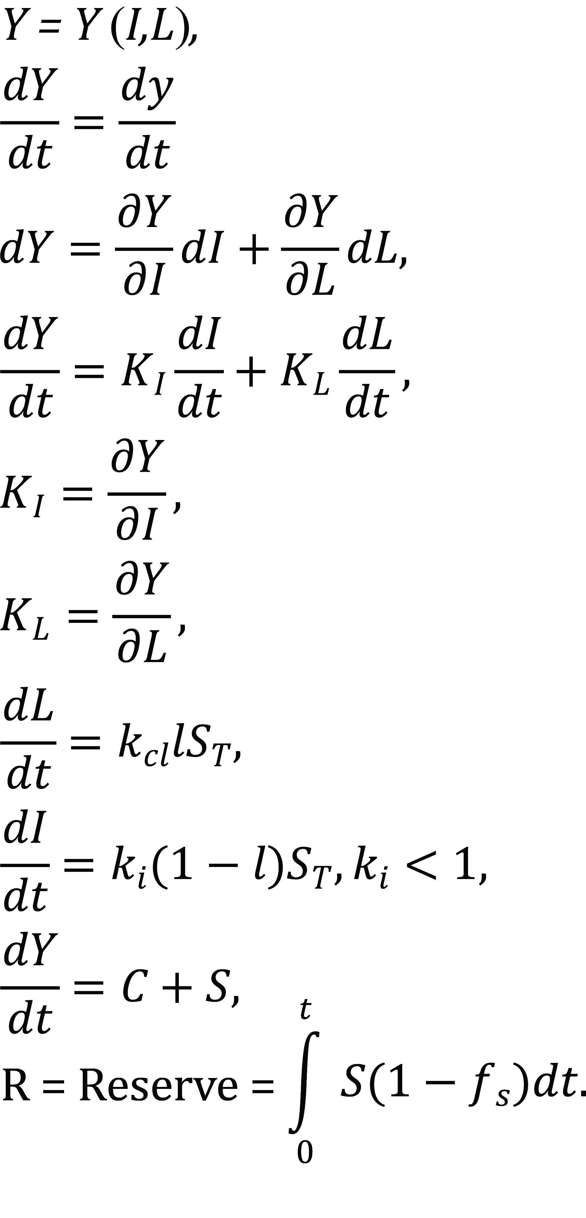
After investment into labor and capital, the output changes as follows:

 

 

Which contributes to consumption and savings. The feedback of change in output (with respect to time) to savings which get invested in production, and productivity of labor and capital are the key determinants of rate of change of output as depicted in the feedback loop of production / output in Figure 1. Production rate equals consumption rate plus saving rate as follows:

 

 

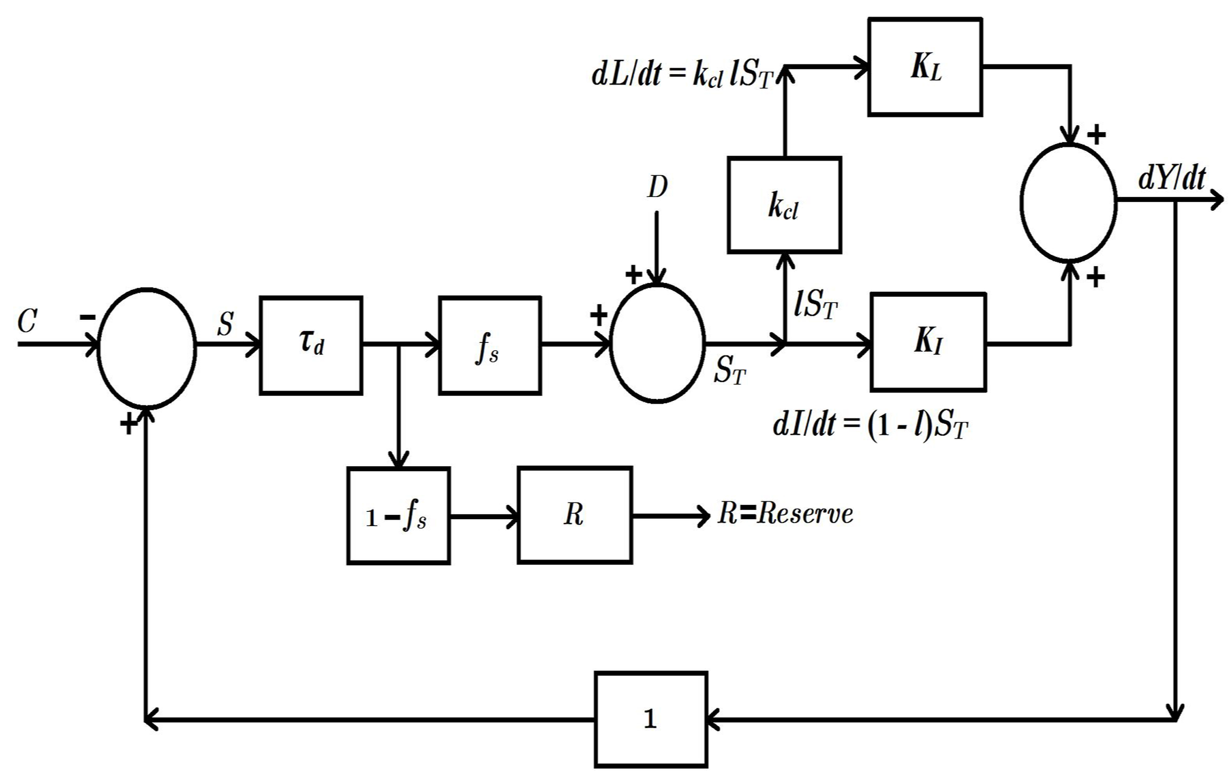
Figure 1. A model of economic growth.

 

Change in labor with respect to time due to investment in labor is as follows:

 

 

Similarly, change in capital with respect to time due to investment in capital is as follows:

 

 

Where ki ˂ 1 takes care of depreciation factor, i.e., only a fraction of amount invested in capital contributes to an increase in capital with respect to time due to depreciation of existing capital, e.g., if an amount of $100 is invested in capital in one time period, however, the existing capital depreciates by $10, then a change in capital is just $90 instead of $100, and ki = 0.9.

 

Substituting Equations (2)-(4) in (1), we obtain:

 

 

Substituting value of ST in above expression, we get:

 

 

Substituting above in Equation (2), we obtain:

 

 

3 SOLUTION OF THE MODEL

We solve the model by assuming exogenous investment input D = 0, i.e., in the absence of capital inflows, foreign remittances, FDI, etc., and the only source of investment in this economy is domestic savings. Let a step input of magnitude A is given to S, i.e., a permanent change in saving rate. The solution (see details in Appendix 1) can be expressed as given below:

 

 

As Y(t) is change in production from steady state, in order to find per capita production, we proceed as follow:

 

 

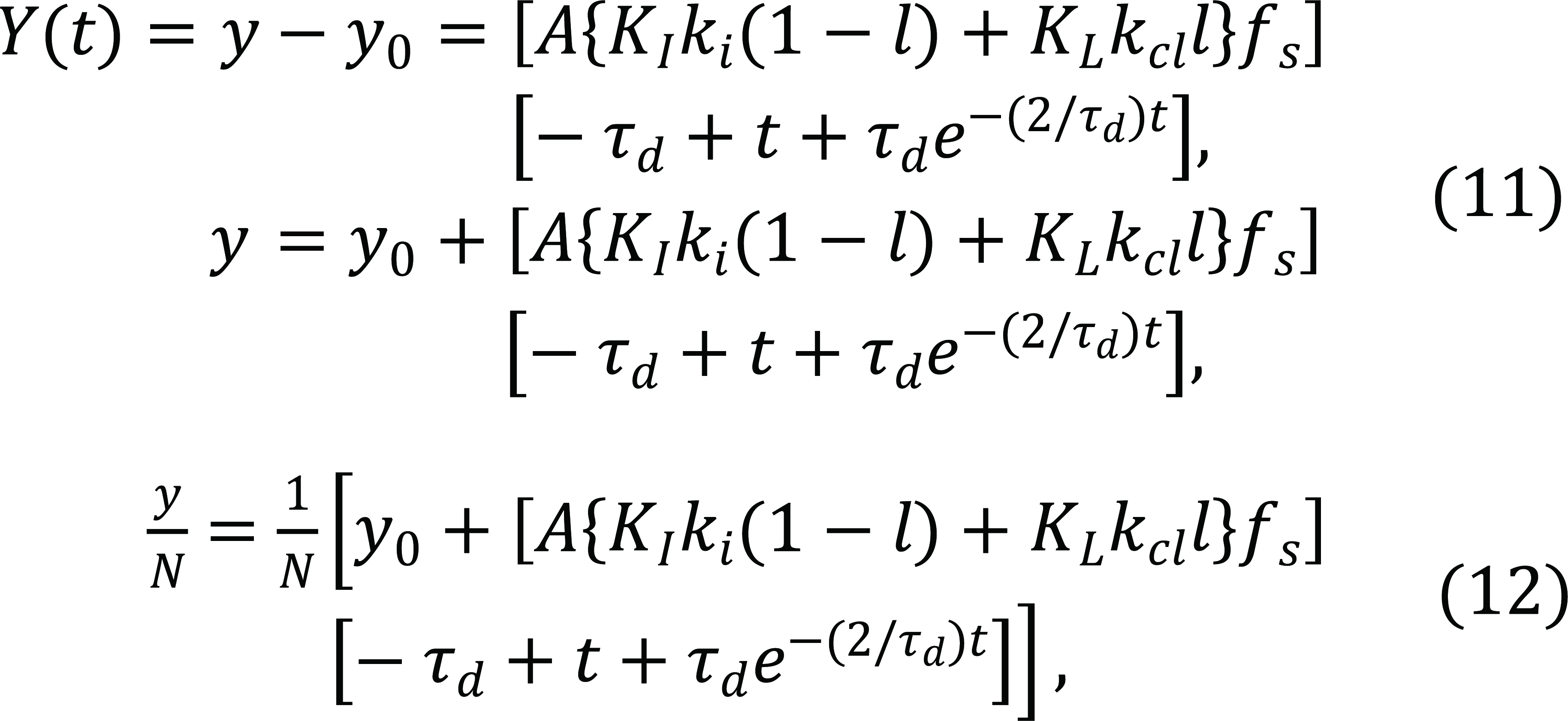
Where N is the population of the country. The condition for per capita growth is as follows:

 

 

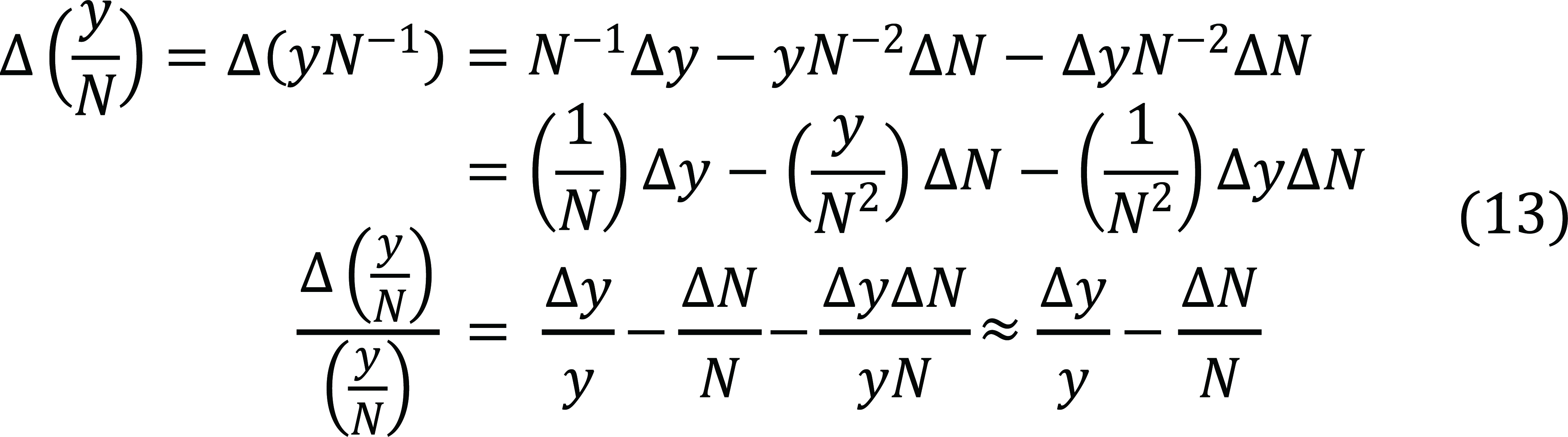
This implies that for a persistent (percent) per capita output / production growth, the percent growth rate of production must be higher than percent population growth, which are both independent of each other, as N does not appear in the expression for y, which is only dependent on fraction of savings invested into labor in addition to other factors, none of which depends on population growth rate. In Equation (11), y, i.e., output / production has two terms depending on time, i.e., t (increasing in time) and e-(2/τd)t (decreasing in time), and the net effect is that the slope of y increases initially due to dead time τd, however, as time increases and approaches infinity, the trend of y becomes linear due to the term t, whereas the term decreasing in time, i.e., e-(2/τd)t approaches zero as t→∞. Depending on the difference trend between values of ∆y/y, and ∆N/N in Equation (13), per capita income of various countries can either converge to a steady state value or diverge, explaining different convergence and divergence patterns across various countries. Technological progress and human capital are captured through productivity parameters of capital and labor, i.e., KI, and KL. Technological progress makes capital more productive; similarly, human capital makes labor more productive. Both parameters appear in the expression for production, i.e., y and are positively related to the output. As technological advancement happens, and a nation invests more in human capital, both these parameters increase in value, hence contributing to an increase in output.

 

3.1 Example 1

In this example the following values have been used for countries 1 and 2 with per capita income Y1t, and Y2t respectively in the Figure 2:

 

For country 1:

y0 = 2, A = 2.3, KI = 1.3, ki = 0.9, l = 0.5, KL = 1.1, dL / dt = 3, fs = 0.2, τd = 5, N = N0(1-e-t), N0 = 80.

For country 2:

y0 = 8, A = 1.5, KI = 1.3, ki = 0.9, l = 0.5, KL = 1.1, dL / dt = 3, fs = 0.2, τd = 5, N = N0(1-e-t), N0 = 80.

 

It is evident from the Figure 2 that both countries have a persistent per capita income growth. Country 1 with much lower, i.e., one fourth initial per capita income not only shows convergence to that of country 2, and rather surpasses that after some time due to higher saving rate.

 

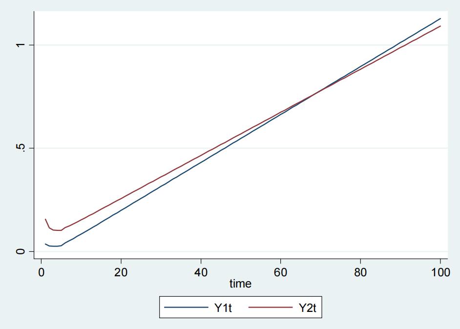
Figure 2. Example 1.

 

3.2 Example 2

In this example the following values have been used for countries 1 and 2 with per capita income Y1t, and Y2t respectively in the Figure 3:

 

For country 1:

y0 = 2, A = 1.5, KI = 1.3, ki = 0.9, l = 0.5, KL = 1.1, dL / dt = 3, fs = 0.2, τd = 5, N = N0(1-e-t), N0 = 80.

For country 2:

y0 = 8, A = 2.3, KI = 1.3, ki = 0.9, l = 0.5, KL = 1.1, dL / dt = 3, fs = 0.2, τd = 5, N = N0(1-e-t), N0 = 80.

 

In example 2, we have just switched the saving rate values for both countries in example 1, and now both countries show a divergence of per capita income instead of convergence.

 

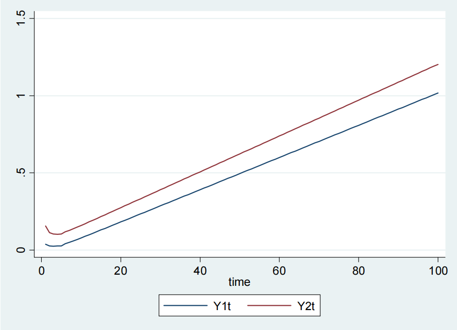
Figure 3. Example 2.

 

3.3 Example 3

In this example the following values have been used for countries 1 and 2 with per capita income Y1t, and Y2t respectively in the Figure 4:

 

For country 1:

y0 = 2, A = 2.3, KI = 1.3, ki = 0.9, l = 0.8, KL = 1.1, dL / dt = 3, fs = 0.2, τd = 5, N = N0(1-e-t), N0 = 80.

For country 2:

y0 = 8, A = 1.5, KI = 1.3, ki = 0.9, l = 0.5, KL = 1.1, dL / dt = 3, fs = 0.2, τd = 5, N = N0(1-e-t), N0 = 80.

 

This example is identical to example 1 with a higher value of l for country 1. It can be seen that when labor has a lower productivity than capital, i.e., KL ˂ KI, then by increasing the fraction of savings going into labor for country 1, i.e., the one with lower initial income shows a divergence of per capita income from that of country 2 in spite of a higher saving rate.

 

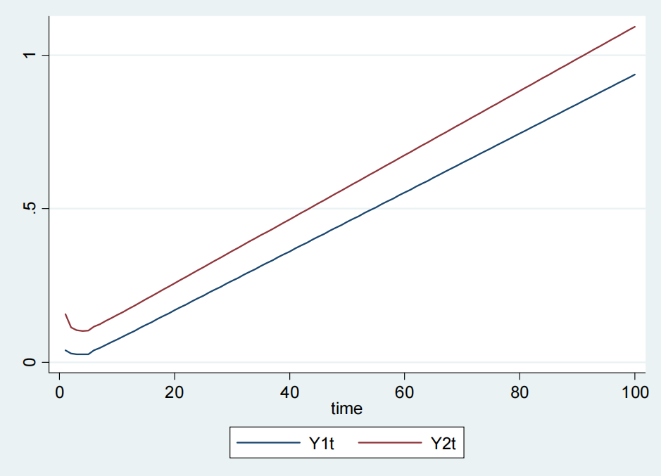
Figure 4. Example 3.

 

3.4 Example 4

In this example the following values have been used for countries 1 and 2 with per capita income Y1t, and Y2t respectively in the Figure 5:

 

For country 1:

y0 = 2, A = 8, KI = 0.5, ki = 0.9, l = 0.8, KL = 2.0, dL / dt = 3, fs = 0.2, τd = 5, N = N0(1-e-t), N0 = 80.

For country 2:

y0 = 8, A = 1, KI = 0.5, ki = 0.9, l = 0.1, KL = 2.0, dL / dt = 3, fs = 0.2, τd = 5, N = N0(1-e-t), N0 = 80.

 

This example shows that when labor productivity is higher than that of labor, i.e., KL ˂ KI for both countries and are equal for both countries, then both countries show a convergence pattern in per capita income if country 1, i.e., the one with lower initial per capita income saves a lot and invests in higher productive labor proportionately more in labor than capital.

 

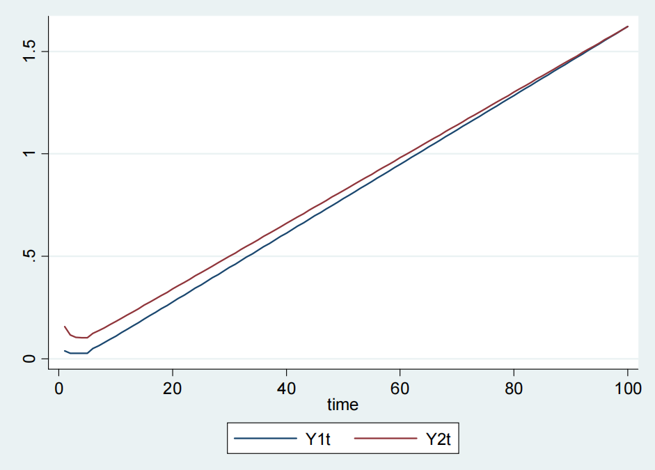
Figure 5. Example 4.

 

There are lots of parameters involved, various combinations of these parameters can explain convergence and divergence patterns across countries. The model has been solved assuming that exogenous investment input D = 0, i.e., in the absence of capital inflows, foreign remittances, FDI, etc., and the only source of investment in this economy is domestic savings. However, when D is not set to zero, the results will get influenced by the presence of external capital inflows / outflows. With D = 0, for a persistent (percent) per capita output / production growth, the percent growth rate of production has to be greater than percent population growth, which are both independent of each other, as N does not appear in the expression for y, which is only dependent on fraction of savings invested into labor in addition to other factors, none of which depends on population growth rate. In Equation (11), y, i.e., output / production invloves two terms depending on time, i.e., t (increasing in time) and e-(2/τd)t (decreasing in time), and the net effect is that the slope of y increases initially due to dead time τd, however, as time increases and approaches infinity, the trend of y becomes linear due to the term t, whereas the term decreasing in time, i.e., e-(2/τd)t approaches zero as t→∞. Depending on the difference trend between values of ∆y/y, and ∆N/N in Equation (13), per capita income of various countries can either converge to a steady state value or diverge, explaining different convergence and divergence patterns across various countries. Technological progress and human capital are captured through productivity parameters of capital and labor, i.e., KI, and KL. Technological progress makes capital more productive; similarly, human capital makes labor more productive. Both parameters appear in the expression for production, i.e., y and are positively related to the output. As technological advancement happens, and a nation invests more in human capital, both these parameters increase in value, resulting in an increase in output.

 

4 CONCLUSION

Countries can achieve a persistent economic growth through saving a fraction of their output and investing that into labor and capital (opposed to the identity savings equal capital investment), a result which contradicts Solow growth model’s conclusion that a change in saving rate has no effect on the rate of growth in the long run; and show a convergence or divergence pattern in per capita income depending on various parameters shown in Equation (12). Output growth for an economy is independent of population growth rate, and rather depends on fractions of savings invested into labor and capital to get more output. It also depends on productivity parameters of capital and labor capturing technological progress and human capital. Technological progress makes capital more productive; similarly, human capital makes labor more productive. Productivity parameters appear in the expression for production, i.e., y and are positively related to the output. As technological advancement happens, and a nation invests more in human capital, both these parameters increase in value, hence contributing to an increase in output. Furthermore, output growth depends on fraction of total amount (savings plus foreign investment available for investing into labor and capital) gone into labor and capital, change in savings rate, and time delay involved in investing savings into capital and labor. A per capita (percent) output growth is possible only if percent change in output is greater than percent change in population. It shows how simply a persistent economic growth (percent increase in output) can be achieved by modeling economic growth with minimum level of assumptions as compared to those in existing literature, based on empirical parameters which can be estimated from real world data, and hence leading to robust results. No restrictions, such as constant returns to scale, etc., have been imposed on production technology. The model does not consider the typical assumption of taking population growth rate as the labor growth rate, and rather assumes that change in labor is dependent on fraction of savings’ feedback to labor instead of all savings contributing to capital. The model predicts convergence of per capita output for countries depending on their parameter values, such as savings fraction invested for more output, labor and capital productivity, population growth rate, etc., and it also predicts divergence for different sets of parameter values for two countries.

 

Acknowledgements

Not applicable.

 

Conflicts of Interest

The authors declared no conflict of interest.

 

Author Contribution

Ahmed MA conceived the main idea of the paper, planned on methodology, did literature review, and sketched outlines of the models. Nawaz N worked on details of the models and derived mathematical results. Both authors jointly prepared the working draft of the article, proofread, and agreed on the final draft for submission to the journal.

 

Abbreviation List

FDI, Foreign direct investment

 

References

[1] Shapirov I. Contemporary economic growth models and theories: A literature review. CES Working Papers, 2015; 7: 759-773.

[2] Solow RM. A contribution to the theory of economic growth. Q J Econ, 1956; 70: 65-94.[DOI]

[3] Solow RM. Technical change and the aggregate production function. Rev Econ Stat, 1957; 39: 312-320.[DOI]

[4] Lucas Jr RE. On the mechanics of economic development. J Monetary Econ, 1988; 22: 3-42.[DOI]

[5] Romer PM. Human capital and growth: Theory and evidence. 1989.

[6] Change ET. Endogenous Technological Change. J Polit Econ, 1990; 98: 2.

[7] Aghion P, Howitt P. A model of growth through creative destruction. 1990.

[8] Grossman GM, Helpman E. Innovation and growth in the global economy. MIT press: Cambridge, USA, 1993.

[9] McDonald S, Roberts J. Growth and multiple forms of human capital in an augmented Solow model: a panel data investigation. Econ Lett, 2002; 74: 271-276.[DOI]

[10] Durlauf SN, Kourtellos A, Minkin A. The local Solow growth model. Eur Econ Rev, 2001; 45: 928-940.[DOI]

[11] Parente S. The failure of endogenous growth. Knowl Tech Policy, 2001; 13: 49-58.[DOI]

[12] Bräuninger M, Pannenberg M. Unemployment and productivity growth: an empirical analysis within an augmented Solow model. Econ Model, 2002; 19: 105-120.[DOI]

[13] Karabona P, Koutun A. An empirical study of the solow growth model. 2013.

[14] Krugman P. The new growth fizzle. New York Times. Available at:[Web]

[15] Onyimadu CO. An overview of endogenous growth models: Theory and critique. Int J Phys Soc Sci, 2015; 5.[DOI]

[16] Chirwa TG, Odhiambo NM. Exogenous and endogenous growth models: A critical review. Comp Econ Res, 2018; 21: 63-84.[DOI]

[17] Ghosh T, Parab PM. Assessing India’s productivity trends and endogenous growth: New evidence from technology, human capital and foreign direct investment. Econ Model, 2021; 97: 182-195.[DOI]

[18] Hac LD, Nguyen Ngoc T. Evaluating Endogenous Growth. J Contemp Iss Bus Gov, 2021; 27.

[19] Bhattacharjee M, Ghosh D. On Dynamics of Economic Development in the Light of Endogenous Growth: A Theoretical and Empirical Investigation. In: Globalization, Income Distribution and Sustainable Development. Emerald Publishing Limited: Leeds, UK, 2022; 21-30.[DOI]

 

Copyright © 2024 The Author(s). This open-access article is licensed under a Creative Commons Attribution 4.0 International License (https://creativecommons.org/licenses/by/4.0), which permits unrestricted use, sharing, adaptation, distribution, and reproduction in any medium, provided the original work is properly cited.