Predicting Crude Oil Price in Nigeria with Machine Learning Models

 

Tayo P Ogundunmade1,2*, Adedayo A Adepoju1, Abdelaziz Allam2

 

1Department of Statistics, University of Ibadan, Ibadan, Nigeria

2Department of Mathematics, University of Tlemcen, Tlemcen, Algeria

 

*Correspondence to: Tayo P Ogundunmade, Masters, Teaching Assistant, Department of Statistics, University of Ibadan, Oduduwa Road, Ibadan, Oyo, 200132, Nigeria; Email: ogundunmadetayo@yahoo.com

 

DOI: 10.53964/mem.2022004

 

Abstract

Background: The rise in crude oil prices yields serious consequences for both oil-producing and non-oil-producing countries. The increase in global commodity prices contributes to the financial income and foreign exchange reserves of oil-exporting countries. However, countries such as Nigeria that sell crude oil and purchase refined fuel confront more complicated situations. To this end, there exists a need to obtain a robust prediction model for the crude oil price of Nigeria.

 

Objective: This study is to determine the best model among the machine-learning time series models considered to predict crude oil prices in Nigeria.

 

Methods: The alternative models were the auto-regressive integrated moving average model, Naive Bayes, Holtwinter trend model, exponential smoothing model, and neural network autoregressive (NNETAR) model. The prediction criteria adopted for model screening were the root mean square error (RMSE), mean absolute error (MAE) and mean absolute percentage error (MAPE). Daily crude oil prices in dollars obtained from the Central Bank of Nigeria were used for analysis spanning from October 1, 2009 to March 22, 2022 with 2836 data points.

 

Results: The NNETAR model showed the minimum RMSE, MAE, and MAPE for cross-validation sets considered.

 

Conclusion: The NNETAR model was recommended for the prediction of crude oil prices in Nigeria.

 

Keywords: crude oil price, prediction, MAPE, artificial neural network, ARIMA

 

1 INTRODUCTION

Crude oil substantially affects financial development, social strength, and public safety worldwide[1]. Over the last two decades, the prediction of crude oil price and its volatility has been heavily studied, as accurate crude oil price prediction contributes to the development of financial planning, control of opportunities in the business sector, and improvement of future development of oil-related enterprises. Besides, the instability of oil prices is central to resource evaluation and resource allocation[2]. Nevertheless, the determination of crude oil prices is difficult[3] and is subject to various factors, such as the fundamental supply-demand relationship and the impact of disease[4].

 

For instance, the COVID-2019 pandemic resulted in the crude oil price tumbling to a notable low on April 20. These factors amplify the prediction uncertainty while compromising prediction accuracy. In light of such vulnerabilities, a superior and more viable strategy for crude oil price prediction is necessitated. Due to the exceptionally nonlinear, unpredictable, and complex attributes of crude oil prices, conventional econometric models fail to perform an accurate prediction. Artificial intelligence algorithms, such as artificial neural networks (ANNs), support vector regression, and least squares support vector regression (LSSVR), have been well recognized for the management of nonlinear and non-stationary time series[5,6].

 

Currently, a plethora of algorithms have been proposed to anticipate crude oil prices. These algorithms, incorporating at least two of the aforementioned models, have been synthesized into three categories, namely, econometric methodologies, artificial intelligence, and crossover models. The autoregressive integrated moving average (ARIMA), random walk, vector autoregression, error correction models (ECM), and generalized autoregressive conditional heteroskedasticity (GARCH) are extensively utilized in forecasting crude oil prices and their volatility[7,8]. For example, ECM is used to investigate the fluctuation of crude oil prices[9], the ARIMA model is to anticipate the Brent crude oil price with a presumption of the availability of the ARIMA (1,1,1) model to foresee the global crude oil prices temporarily[10], and the capacity of short-memory multivariate GARCH models and long-memory multivariate models to anticipate unrefined petroleum information is analyzed, with the assumption that long-memory multivariate models outperform short-memory multivariate models[8]. Wang et al.[11] examined the foresight of univariate and multivariate GARCH-class models with energy market instability and found that univariate models with asymmetric effects outflanked others. The research by Klein et al.[12] showed that the mixed memory GARCH (MMGARCH) outperformed other models in anticipating unpredictability and opportunity worth (GARCH, EGARCH, and APARCH, among others).

 

To avoid the weaknesses of traditional financial models that assume linearity of the data being processed, several nonlinear and artificial intelligence models have received extensive attention in crude oil price forecasting. Artificial neural networks (ANNs), support vector machines, and least squares support vector regression (LSSVR) are the most widely used artificial intelligence algorithms[13-17]. An adaptive model was proposed in view of ANNs to anticipate long-term oil costs[18], in which crude oil news is used to forecast crude oil costs with success. Moreover, text features were extracted from online crude oil news using a convolutional neural network to demonstrate the explanatory power of crude oil price prediction[19]. The objective of the present study is to determine the best model for predicting crude oil prices in Nigeria among the considered machine learning time series models.

 

2 MATERIALS AND METHODS

Time series models, such as the ARIMA model, simple exponential smoothing, naïve forecasting method, Holtwinter’s trend model, and neural network autoregressive (NNETAR) model, were adopted for analysis.

 

2.1 Data Extraction

The data used herein were the daily data of crude oil prices obtained from the Central Bank of Nigeria spanning from October 1, 2009 to March 22, 2022 totaling 2836 data points.

 

2.2 Arima

The ARIMA model was used for time series data analyses. The autoregressive (AR) and moving average (MA) models were jointly employed for stationary data analyses. The order of the ARIMA model was typically denoted as ARIMA (p, d, q), where “d” represents the difference frequency used to render the data stationary, “p” represents the number of spikes across the significant line of the partial autocorrelation function (PACF) plot, and “q” represents the number of spikes across the significant line of the autocorrelation function (ACF) plot. To test for stationarity, the augmented dickey fuller, Phillips-Perron, and KPSS tests with trends and an intercept were incorporated. The ARIMA (p, d, q) model was given, with time series data Xt :

 

 

the AR component of the model is Ø(B) which is the characteristic polynomial of order ‘p’;

the MA component of the model is Ɵ(B) which is the characteristic polynomial of order ‘q’,

the difference in order ‘d’ of the data is (1-B)d,

Xt is the observed value at time t,

Zt is the random error associated with observation at time t.

 

Using the Akaike Information Criterion (AIC), the model derived from inspecting the ACF and PACF plots was compared to models with similar parameters to identify a better model.

 

2.3 Naïve Forecasting Method

Naive forecasting is a technique in which the values of the previous period are used to predict the next period without predictions or adjustment factors, and the formula is as follows.

 

 

The Naive forecasting method is one of the simplest of all forecasting methods.

 

2.4 Simple Exponential Smoothing

Rather than a simple average that is used as the basis for the next forecast, it weights exponents decreasingly based on external factors, which is to 'smooth' out the averages and produce a more reliable forecast. Exponential smoothing is the use of an exponentially weighted moving average (EWMA) to “smooth” a time series. A new time series st that is a smoothed version of xt was defined, with a time series xt as:

 

 

2.5 Holtwinters Trend Model

Holt-Winters is a method to model three aspects of the time series: a typical value (average), a slope (trend) over time, and a cyclical repeating pattern (seasonality).

 

To account for a linear trend, the simple exponential smoothing model was modified, which is termed Holt’s exponential smoothing and consists of two EWMAs, the smoothed xt value and its slope.

 

 

 

In addition, the term for the slope needs to be accounted for in the prediction. To predict the value of m future time steps, Ft+m was used as the formula for the m-step-ahead forecast, given as:

 

 

2.6 NNETAR Model

ANN is a computational model based entirely on the shape and capabilities of biological neural networks. ANNs are nonlinear statistical information modeling tools used to model complex relationships between inputs and outputs or to determine patterns. ANNs have three layers that may or may not be interconnected. The first layer is composed of input neurons. The first layer neurons send data directly to the second layer, and the output neurons are then sent to the third layer. Neural networks typically have one input layer, one output layer, and several hidden layers between the input and output layers. Each layer consists of weights and biases. 70% of the data is used for the training set, while 30% is used as the testing set.

 

Feedforward neural network: A feedforward neural network is a biologically inspired classification algorithm. It is composed of several simple neuron-like processing units that are arranged in layers. Every unit in a layer is related to every unit in the previous layer. It is the most basic type of neural network. The tangent hyperbolic (Tanh) activation function is used. The mathematical representation of the ANN model is given as:

 

 

Where,

y: crude oil price;

wjh: weight from the input to hidden nodes;

wh: weight from the hidden to output node;

yi-1: lag of the y;

α, αh: bias;

Φ0, Φh: activation functions.

 

2.7 Performance Measures

Three criteria were used in this study to assess the performance of the models.

 

The root mean squared error (RMSE) is a commonly used measure of the difference between the value predicted by a model and the observed value. The RMSE denotes the square root of the second sample moment of the difference between the predicted and observed values or the quadratic mean of these differences. These deviations are referred to as residuals when calculated for the sample of data used for estimation and as errors (or prediction errors) when calculated out-of-sample.

 

The difference between two continuous variables is referred to as the mean absolute error (MAE).

 

MAE is a measure of the error between pairwise observations that express the same phenomenon by calculating the average magnitude of the error without considering the direction of magnitude.

The mean absolute percentage error (MAPE) measures the accuracy of a forecasting method's prediction. It expresses the accuracy as a ratio.

 

Mathematically, it is defined by the following formulas:

 

 

 

 

 

3 RESULTS AND DISCUSSION

The stationarity of the time series data was done using the Augmented dickey fuller test, Phillips-Perron unit root test, and KPSS unit root test. The machine learning models considered are the ARIMA model, simple exponential smoothing, naïve forecasting method, Holtwinters trend model, and NNETAR model. The models were analyzed and compared using training sets of 70, 80, and 90.

 

Figure 1 shows the descriptive statistics of the crude oil price data. The summary report for crude oil price shows the histogram, Anderson-Darling normality test, and descriptive statistics including mean, standard deviation, variance, skewness, kurtosis, minimum, 1st quartile, median, 3rd quartile, and maximum values. The report also shows the 95% confidence interval for the means and medians. The results show that crude oil prices in dollars have a mean of 76.766, a standard deviation of 27.427, a variance of 752.267, a skewness of 0.16272, and a kurtosis -1.08975, respectively. The minimum, 1st quartile, median, 3rd quartile, and maximum values are 7.150, 54.500, 72.410, 107.120, and 139.410, respectively. Figure 1 also presents the histogram of the crude oil price data.

 

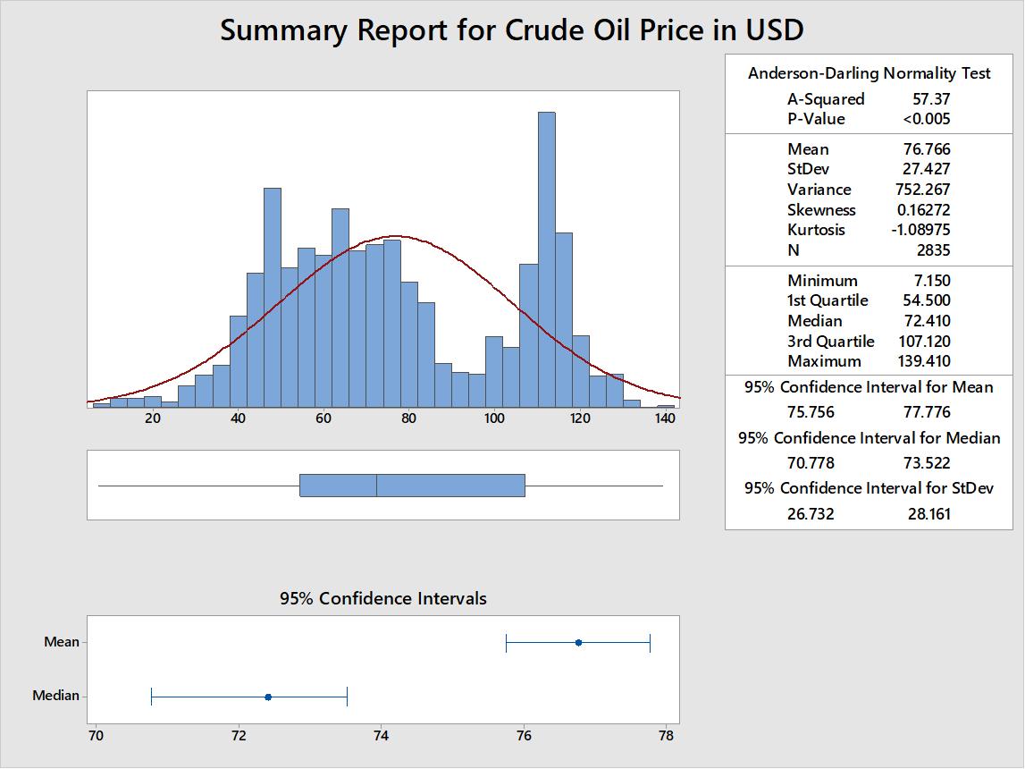
Figure 1. Summary report for crude oil prices.

 

3.1 Time Plot and Stationarity Test

Unit root test shows the stationarity status of the data. Augmented Dickey-Fuller test, Phillips-Perron unit root test, and KPSS unit root test are the unit root test approaches used to test the stationarity of the crude oil prices. The results show that crude oil prices are stationary with drift and trend with a significant value of less than 5% level of significance.

 

The results in Table 1, Table 2, and Table 4 show that the p-value for time series is greater than 0.05, indicating failure in rejecting the null hypothesis and non-stationary time series. While Tables 3 and 5 show a significant p-values. The rejection of the trend hypothesis implies a high likelihood of no unit root and a trend stationary process.

 

Table 1. Augmented Dickey-Fuller Test without Drift and Trend

 

Table 2. Augmented Dickey-Fuller Test without Trend but Drift

 

Table 3. Augmented Dickey-Fuller Test with Drift and Trend

Note: P value=0.95 means P value≤0.05.

 

Table 4. Phillips-Perron Unit Root Test

Note: P value=0.01 means P value≤0.01.

 

Table 5. KPSS Unit Root Test

 Note: P value=0.10 means P value≥0.10.

 

3.1.3 Trend Analysis

Trend analysis was performed on the crude oil price data to obtain the predictive performance of the linear trend analysis. Figure 2 exhibits that the linear trend analysis computed using the crude oil price data is given as

 

 

This implies that the crude oil prices in dollars will produce a positive value of 104.539 when there is no contribution. In addition, the linear equation implies a negative correlation between time and crude oil prices in dollars. In each unit of time, the crude oil prices in dollars decrease by 0.019586. Predictions are available using the above linear trend equation.

 

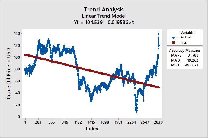
Figure 2. Trend analysis plot for crude oil prices.

 

3.2 Performance Measures Result

The data were divided into training sets of 70, 80, and 90 percent respectively. The results in Tables 6-8 show the MAPE, MAE, and RMSE for the forecast performance of the models.

 

Table 6. Models Performance at Training Set of 70%

 

Table 7. Models Performance at Training Set of 80%

 

Table 8. Models Performance at Training Set of 90%

 

The performance of these models in the cross-validation of 70%, 80%, and 90% training sets using MAPE, MAE, and RMSE as the performance criteria are presented in Tables 6-8. A closer inspection of these tables reveals that these models produce MAPE, MAE, and RMSE for the NNETAR model in all training sets (70, 80, and 90).

 

4 CONCLUSION

In this work, modeling of crude oil prices is available using the ARIMA model, simple exponential smoothing, naïve forecasting method, Holtwinters trend model, and NNETAR model. Stationarity tests of data with trends were obtained using the augmented dickey fuller unit root test, Phillip-Perron unit root test, and the KPSS unit root test. The results demonstrated that the data were stationary when drift and trend were incorporated. A linear trend model was obtained from the data using time as the dependent variable, which allows a valid prediction of the crude oil prices in Nigeria. Furthermore, among the five models considered, the NNETAR model yielded the optimal forecast performance for crude oil prices in Nigeria as it had the lowest RMSE and the MAE among all other models. Thus, the NNETAR model was recommended for the prediction of crude oil prices in Nigeria. Further study can be done by incorporating crude oil price interventions over years to understand the price changes.

 

Acknowledgments

Not Applicable.

 

Conflicts of Interest

The authors had no conflict of interest.

 

Author Contribution

Ogundunmade TP designed this study and wrote this article. Adepoju AA and Allam A revised the paper for intellectual content. All authors approved the final version.

 

Abbreviation List

ACF, Autocorrelation function

ANNs, Artificial neural networks

AR, Autoregressive

ARIMA, Autoregressive integrated moving average

ECM, Error correction models

EWMA, Exponentially weighted moving average

GARCH, Generalized autoregressive conditional heteroskedasticity

LSSVR, Least squares support vector regression

MA, Moving average

MAE, Mean absolute error

MAPE, Mean absolute percentage error

NNETAR, Neural network autoregressive

PACF, Partial autocorrelation function

RMSE, Root mean square error

 

References

[1] Wu G, Zhang YJ. Does China factor matter? An econometric analysis of international crude oil prices. Energ Policy, 2014; 72: 78-86. DOI: 10.1016/j.enpol.2014.04.026

[2] Zhao Y, Li J, Yu L. A deep learning ensemble approach for crude oil price forecasting. Energ Econ, 2017; 66: 9-16. DOI: 10.1016/j.eneco.2017.05.023

[3] Yu L, Zhao Y, Tang L. Ensemble forecasting for complex time series using sparse representation and neural networks. J Forecasting, 2017; 36: 122-138. DOI: 10.1002/for.2418

[4] Monge M, Gil-Alana LA, de Gracia FP. Crude oil price behaviour before and after military conflicts and geopolitical events. Energ, 2017; 120: 79-91. DOI: 10.1016/j.energy.2016.12.102

[5] Lahmiri S. Comparing variational and empirical mode decomposition in forecasting day-ahead energy prices. IEEE Syst J, 2015; 11: 1907-1910. DOI: 10.1109/JSYST.2015.2487339

[6] Li SR, Ge YL. Crude oil price prediction based on a dynamic correcting support vector regression machine. Abstr Appl Anal, 2013; 2013: 666-686. DOI: 10.1155/2013/528678

[7] Lin L, Jiang Y, Xiao H et al. Crude oil price forecasting based on a novel hybrid long memory GARCH-M and wavelet analysis model. Physica A, 2020; 543: 123532. DOI: 10.1016/j.physa.2019.123532

[8] Marchese M, Kyriakou I, Tamvakis M et al. Forecasting crude oil and refined products volatilities and correlations: New evidence from fractionally integrated multivariate GARCH models. Energ Econ, 2020; 88: 104757. DOI: 10.1016/j.eneco.2020.104757

[9] Kanjilal K, Ghosh S. Dynamics of crude oil and gold price post 2008 global financial crisis-New evidence from threshold vector error-correction model. Resour Policy, 2017; 52: 358-365. DOI: 10.1016/j.resourpol.2017.04.001

[10] Xiang Y, Zhuang XH. Application of ARIMA model in short-term prediction of international crude oil price. Adv Mater Res, 2013; 798: 979-982. DOI: 10.4028/www.scientific.net/AMR.798-799.979

[11] Wang Y, Wu C. Forecasting energy market volatility using GARCH models: Can multivariate models beat univariate models? Energ Econ, 2012; 34: 2167-2181. DOI: 10.1016/j.eneco.2012.03.010

[12] Klein T, Walther T. Oil price volatility forecast with mixture memory GARCH. Energ Econ, 2016; 58: 46-58. DOI: 10.1016/j.eneco.2016.06.004

[13] Hu H, Wang L, Lv SX. Forecasting energy consumption and wind power generation using deep echo state network. Renew Energ, 2020; 154: 598-613. DOI: 10.1016/j.renene.2020.03.042

[14] Huang L, Wang J. Global crude oil price prediction and synchronization based accuracy evaluation using random wavelet neural network. Energ, 2018; 151: 875-888. DOI: 10.1016/j.energy.2018.03.099

[15] Wu B, Wang L, Wang S et al. Forecasting the US oil markets based on social media information during the COVID-19 pandemic. Energy, 2021; 226: 120403. DOI: 10.1016/j.energy.2021.120403

[16] Ogundunmade TP, Adepoju AA. The performance of artificial neural network using heterogeneous transfer functions. Int J Data Sci, 2021; 2: 92-103. DOI: 10.18517/ijods.2.2.92-103.2021

[17] Ogundunmade TP, Adepoju AA. On heterogenous transfer functions in bayesian neural network. Paper presented at the Virtual Paper Session-16th Brazilian Meeting of Bayesian Statistics and VI Latin American Conference on Statistical Computing, March, 2022.

[18] Azadeh A, Moghaddam M, Khakzad M et al. A flexible neural network-fuzzy mathematical programming algorithm for improvement of oil price estimation and forecasting. Comput Ind Eng, 2012; 62: 421-430. DOI: 10.1016/j.cie.2011.06.019

[19] Wu B, Wang L, Lv SX et al. Effective crude oil price forecasting using new text-based and big-data-driven model. Measurement, 2021; 168: 108468. DOI: 10.1016/j.measurement.2020.108468

 

Copyright © 2022 The Author(s). This open-access article is licensed under a Creative Commons Attribution 4.0 International License (https://creativecommons.org/licenses/by/4.0), which permits unrestricted use, sharing, adaptation, distribution, and reproduction in any medium, provided the original work is properly cited.