Jerk and Energy Issues in Optimal Trajectory Planning for Robot Manipulators

 

Atef A. Ata1*

 

1Department of Engineering Mathematics and Physics, Faculty of Engineering, Alexandria University, Alexandria, Egypt

 

*Correspondence to: Atef A. Ata, PhD, Professor, Department of Engineering Mathematics and Physics, Faculty of Engineering, Alexandria University, 22 El-Guish Road, Alexandria, 21544, Egypt; Email: atefa@alexu.edu.eg

 

DOI: 10.53964/jmim.2024001

 

Abstract

Objective: One of the important objectives in industrial applications is minimizing the consumed energy due to the unsecured supply lines because of the international crisis and the sudden increase in the prices of the crude oil as well. It is the objective of this research to investigate the effect of jerk and the minimum energy consumption per cycle of the manipulator’s actuators on the optimal trajectory of industrial manipulator.

 

Methods: The design for optimal trajectory for industrial robots has a primary importance in attaining mass production with accurate performance. Optimal trajectory can be designed from start to goal positions to achieve certain criterion optimally such as minimum time, minimum distance and / or minimum energy consumption while avoiding obstacles during the course of motion.

 

Results: The proposed analysis will consider also the jerk which is the time derivative of the acceleration to guarantee that the end-effector will not vibrate at the start and goal of each stroke. A polynomial of seven-degree is proposed to investigate how the jerk affects the optimality of the trajectory and the torques of the joints as well.

 

Conclusion: From the presented parametric study and analysis, it is recommended to apply energy per cycle as a criterion for minimum kinetic energy of an industrial manipulator trajectory in spatial manoeuvring.

 

Keywords: torque, modelling, optimization, industrial, DC motor

 

1 INTRODUCTION

Trajectory planning for manipulator joints can be achieved by many options such as polynomial of different orders, trigonometric functions and Gaussian velocity profile. Researches prefer polynomial simply because its continuity in velocity, acceleration and jerk according to the order of polynomials. On the other hand, polynomial trajectories enable controlling many important variables, for third-order polynomial one can control only the velocity but for fifth-order polynomial one can control the velocity and acceleration as well. If one applies seventh-order polynomial, the jerk can be controlled easily. In engineering applications where robot motion with sudden changes of jerk is not desirable, such as in transferring of people and goods where dropouts and breakages may easily occur. Also, since jerk control coincides with torque rate control, jerk-bounded trajectories result in much smoother actuator loads[1]. It should be noted that planning the robot trajectory using energetic criteria provides several advantages. It yields smooth trajectories resulting easier to track and reducing the stresses to the actuators and to the manipulator structure. The positive effect induced by minimum jerk is high coordinated and smooth robot motion from start to goal[2].

 

The problem of how the jerk affects the trajectory and the required torque by the actuator in conducting tasks has been investigated by eminent researchers. Piazzi and Visioli[3] in 2000 investigated the global constrained minimax problem in order to get the minimum jerk cubic spline trajectories based on interval analysis. In order to prove their findings, they validated their algorithm using six degrees of freedom manipulator and they compared the results with the trigonometric trajectories.

 

In 2003, an online optimal trajectory generator for a smooth jerk-bounded trajectory for industrial robot applications was developed[4]. They used concatenation of fifth-order polynomial between two via points to achieve a linear segment with parabolic blends (LSPB) trajectory. They used a sine wave template to calculate the control points for acceleration ramps. Their approach requires only the computation of a maximum of eight quantic control points for each trajectory. They also verified their approach through both simulation and experiment. A soft motion, jerk-limited optimal trajectory generator for multiple degrees-of-freedom (DOF) surgical robots was presented[5]. They proposed a seven-cubic splines trajectory suitable for service robotics, such as the surgical and nursing robots. The problem of continuity of position, velocity, acceleration, and jerk of electric actuators using two approaches was investigated[6]. Their first approach separates a planned path and a corresponding velocity profile, while the second method combines a fifth-order polynomial trajectory. They validated their approach using a benchmark trajectory of a three DOF planar articulated structure robot and presented a comparison of the two approaches’ results.

 

In 2015 an algorithm for a smooth jerky trajectory bounded in velocity, acceleration and jerk which is suitable for high DOF manipulators with soft motion shortcuts was presented[7]. Their main objective is to shorten the execution time as much as possible while maintaining the feasibility. A smooth speed reference generation algorithm using fifth-order polynomial function for electric actuators was proposed by Park et al[8]. They applied a simple jerk-bounded and time-optimal velocity trajectories with lower computational burden. They validated their algorithm through three case studies with different combinations of the maximum velocity and acceleration.

 

Some researchers tried to develop jerk-bounded trajectories since jerk limitation is vital in industrial manipulator applications to improve path tracking and reduce wear of the robot joints. Bilal et al.[9] investigated the trajectory tracking and vibration control of rotary flexible joint manipulator with parametric uncertainties. The equation of motion for a single link flexible joint manipulator is derived using Lagrange-Euler equation. They applied concatenation of fifth-order polynomial to obtain a smooth trajectory between two via points. They verified their approach numerically by comparison with other trajectories such as cubic spline and LSPB and experimentally on Quansar’s flexible joint manipulator.

 

The structure of this research is as follows: Section 2 explores the trajectory planning as a seventh-order polynomial. Section 3 analyses the energy consumption per cycle for a DC motor and how it can be related to the angular acceleration. Section 4 shows a case study for a 3 DOF robotic arm in spatial motion. Section 5 highlights the discussion and conclusion. It should be mentioning that this paper is an extension of the conference paper[10] and it has more details, analysis, figures and conclusion.

 

2 TRAJECTORY PLANNING

In general, a spline is a polynomial of a degree k with continuity of derivative of order k-1, at the interpolation points. Low-degree polynomials reduce the effort of computations and the possibility of numerical instability[11]. On the other hand, higher-order polynomials enable the control of other variables such as angular acceleration and jerk.

 

A cubic trajectory gives continuous positions and velocities at the start and finish points but discontinuities in the acceleration and potentially, infinite jerk, at trajectory via points. A discontinuity in acceleration leads to impulsive jerk, which may excite the vibrational modes in the manipulator and reduce tracking accuracy. For this reason, one may wish to specify constraints on the acceleration and jerk as well[12].

 

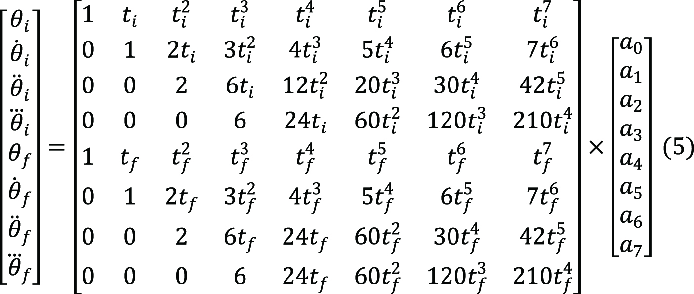
To investigate the jerk effect on the motor torque and the energy consumption of the robot, the trajectory is assumed as a polynomial of 7th order according to the equation:

 

 

Equations (1)-(4) represent the position θ(t), velocity , acceleration , and jerk , of the proposed trajectory respectively, ti and tf are the initial and final time of the proposed trajectory and a0, a1, a2, a3, a4, a5, a6, a7 are coefficients that can be determined from the initial conditions as follows:

 

Once the final travelling time of motion has been fixed, reducing the jerk is required since it reduces the actuator and mechanical strain and the joint wear. This ensures improving trajectory tracking performance by the robot control system and there is also a positive effect on the robot lifespan[3].

 

3 ENERGY CONSUMPTION PER CYCLE

For the schematic diagram of the DC motor illustrated in Figure 1 where: v(t), vb(t), Ra, ia, La, KT, Td(t), Tm(t) and θm, are the input voltage signal, the back electromotive force voltage, the circuit resistance, the armature current, the armature inductance, the back emf constant, disturbance torque, motor torque and the rotor angle position, respectively.

 

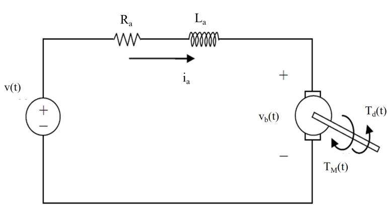
Figure 1. Schematic diagram of a DC motor.

 

Normally, there is a linear relation between the torque of the motor and the armature current ia as:

 

While the back emf is proportional to the angular speed and is given by:

 

Applying Kirchhoff’s law on the electric circuit one gets:

 

Assume that Td represents the disturbance torque, applying Newton’s second law of motion, gives:

in which I is the motor inertia and is the damping torque. For many engineering practices, the damping coefficient c is considered small, then the second equation becomes[13]:

 

The consumed energy per cycle E can be identified as the energy dissipated in the motor resistance R during the time 0≤t≤tf and can be evaluated as:

 

Upon substituting for armature current i from Equation (10) into Equation (11), yields:

 

The right-hand side of Equation (12) has three terms, the first integral is independent of Td and is the energy dissipation when no coulomb friction or load disturbance exists. If Td is constant, the second integral becomes . This is simply because for rest-to-rest maneuvering which we assumed here, the angular velocity vanishes at the start and end of the assumed trajectory. Then the energy dissipated per cycle is given by the first and last terms as:

 

Equation (13) indicates that if Td is constant, its effect on the energy dissipation is negligible. Thus, to find the optimal velocity profile we need only to consider the first term in Equation (12) as a measure for the energy dissipated per cycle.

 

The next objective is to investigate the effect of the jerk in the trajectory by applying the energy per cycle as a criterion to select the optimal trajectory. The initial conditions will be assumed to calculate the coefficients in the trajectory of Equations (1)-(4). The initial and final values of the angle, velocity and acceleration are assumed zero. The final angles are assumed as π/4, π/3 and π/2 and the jerk value at the beginning and end of trajectories are assumed the same for symmetry and their values are changing from zero to 5. Due to this assumption, reference trajectories became symmetric which guarantees the reduction of the computational loads[8]. This approach is not limited to the zero terminal values and it can be extended if the velocity and acceleration values at the terminal points are not trivial. The required values of the boundary conditions can be inserted to find the trajectory coefficients. The results are shown in Table 1 while the optimum trajectories for the three joints based on minimum energy per cycle are presented in Figure 2. Figure 3 shows the relation between jerk and the energy per cycle for the three joints trajectories.

 

Table 1. Energy Per Cycle for the Robot Joints

 

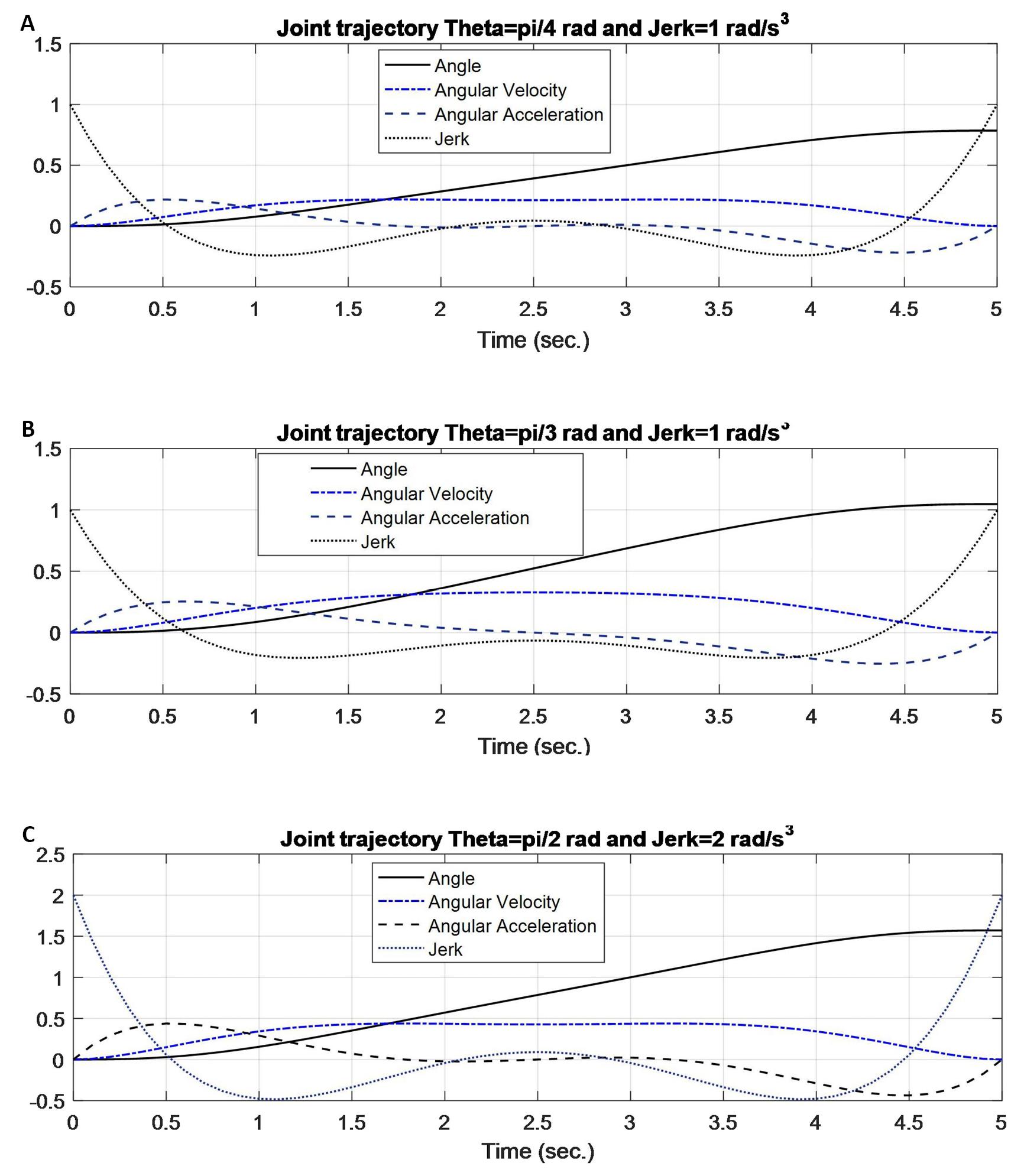
Figure 2. The optimum trajectories for the three joints based on minimum energy per cycle. A: Joint 1 trajectory; B: Joint 2 trajectory; C: Joint 3 trajectory.

 

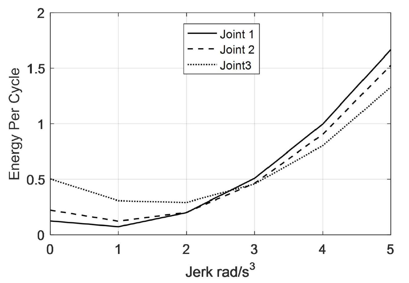
Figure 3. Relation between jerk and energy per cycle.

 

From Figure 3 it is clear that the energy per cycle decreases for low jerk values (Jerk=0 till 3rad/s3) and then increases rapidly after that for the three trajectories. The trend is the same for the three trajectories and this measure can be considered as a basis for selecting the jerk-bounded trajectories for the robot manipulators.

 

4 CASE STUDY

Consider a 3 DOF planar robot arm as shown in Figure 4. The robot moves in the vertical plane so the gravity effect will be included in the analysis. The required equations of motion for the three links can be determined using Lagrange-Euler technique are given in[14]:

 

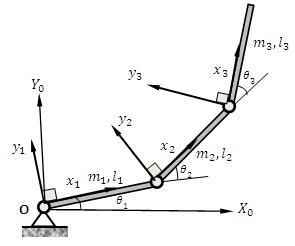
Figure 4. Three DOF planar robotic arm.

 

The equations of motion for a multi-degree of freedom robot with i links and j joints can be given in compact from as:

 

Where:

 

The first term in Equation (14) is the angular acceleration-inertia terms, the second term is the actuator inertia term, the third term is the Coriolis and Centrifugal terms and the last term is the gravity term. For more details regarding the derivation of the equations of motion the reader is referred to Ata et al[14].

 

Upon substituting of the joints trajectories into the equations of motion with the robot parameters as: m1=m2=m3=2kg and l1=l2=l3=0.5m, and I1act.=I2act.=I3act.=0.1kgm2. The joints torques are simulated in Figure 5.

 

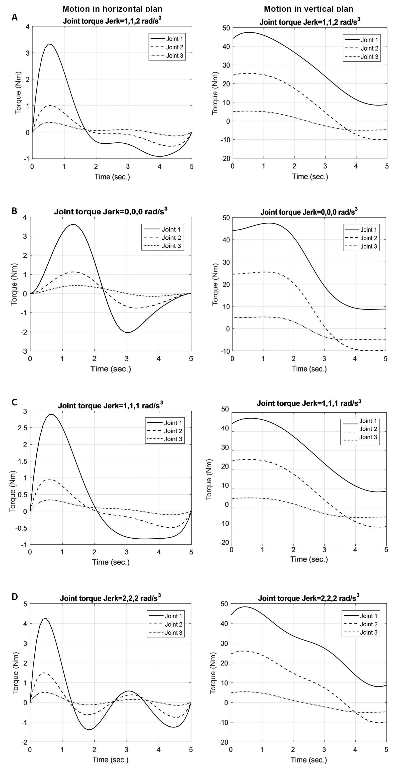
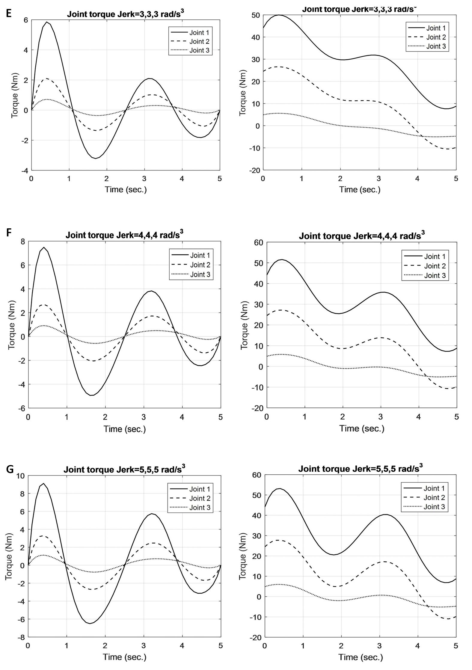
Figure 5. The joints torques. A: Joint torque jerk=1,1,2rad/s3; B: Joint torque jerk=0,0,0rad/s3; C: Joint torque jerk=1,1,1rad/s3; D: Joint torque jerk=2,2,2rad/s3; E: Joint torque jerk=3,3,3rad/s3; F: Joint torque jerk=4,4,4rad/s3; G: Joint torque jerk=5,5,5rad/s3.

 

The joints torque for the assumed three joints for different proposed values of the jerk as well as the optimum jerk values for the horizontal and vertical motion of the robot arm are shown in Table 2.

 

Table 2. Joints Torque for Different Values of the Jerk

 

5 DISCUSSION AND CONCLUSION

The effect of jerk and the energy per cycle on the polynomial trajectory of manipulators are investigated here. It is clear from Figure 5 and from Table 2 that there are two sets of jerks that produce the lowest torque for the three joints in both horizontal and vertical motion of the manipulator. These two sets are the optimum case (the last row of each joint) and the second row of each joint. These two sets are identical except for the jerk value of the last joint trajectory of the manipulator. This is simply because the energy consumption per cycle for joint 3 is similar for the two jerk values of 1 and 2 as can be seen from Table 1. When the jerk increases, the corresponding torque for each joint increases as well. This proves that it is wise to use the energy consumption per cycle as a measure in determining the optimal polynomial trajectory for the robot joints.

 

Acknowledgements

Not applicable.

 

Conflicts of Interest

The author declared no conflict of interest.

 

Author Contribution

Ata AA solely contributed to the manuscript and approved the final version.

 

Abbreviation List

DOF, Degrees-of-freedom

LSPB, Linear segment with parabolic blends

 

References

[1] Kyriakopoulos KJ, Saridis GN. 1988. Minimum jerk path generation. IEEE International Conference on Robotics and Automation (ICRA). Shanghai, China, 24-29 April 1988.[DOI]

[2] Gasparetto A, Zanotto V. A new method for smooth trajectory planning of robot manipulators. Mech Mach Theory, 2007; 42: 455-471.[DOI]

[3] Piazzi A, Visioli A. Global minimum-jerk trajectory planning of robot manipulators. IEEE T Ind Electron, 2000; 47: 140-149.[DOI]

[4] Macfarlane S, Croft EA. Jerk-bounded manipulator trajectory planning: design for real-time applications. IEEE T Robot Autom, 2003; 19: 42-52.[DOI]

[5] Broquere X, Sidobre D, Herrera-Aguilar I. Soft motion trajectory planner for service manipulator robot. 2008 IEEE/RSJ International Conference on Intelligent Robots and Systems. Nice, France, 14 October 2008.[DOI]

[6] Konjević B, Kovačić Z. Continuous Jerk Trajectory Planning Algorithm. The 8th International Conference on Informatics in Control, Automation and Robotics. Noordwijkerhout, Netherlands, 2011.[DOI]

[7] Zhao R, Sidobre D. Trajectory smoothing using jerk bounded shortcuts for service manipulator robots. 2015 IEEE/RSJ International Conference on Intelligent Robots and Systems (IROS). Hamburg, Germany, 28 September 2015 - 2 October 2015.[DOI]

[8] Park BJ, Lee HJ, Oh KK et al. Jerk-Limited Time-Optimal Reference Trajectory Generation for Robot Actuators. Int J Fuzzy Log Intell Syst, 2017; 17: 264-271.[DOI]

[9] Bilal H. Yin B, Kumar A et al. Jerk-bounded trajectory planning for rotary flexible joint manipulator: an experimental approach. Soft Comput, 2023; 27: 4029-4039.[DOI]

[10] Ata AA. Energy Consumption-Based Trajectory Planning for Manipulators. Advances in Manufacturing Technology XXXV: Proceedings of the 19th International Conference on Manufacturing Research, Incorporating the 36th National Conference on Manufacturing Research. Derby, UK, 6-8 September 2022.[DOI]

[11] Fu KS, Gonzalez RC, Lee CSG. Robotics: Control, Sensing, Vision and Intelligence. McGraw-Hill Book Company: Singapore, 1987.

[12] Spong MW, Hutchinson S, Vidyasagar M. Robot Modelling and Control, 1st ed. John Wiley & Sons, Inc.: New York, USA, 2006.

[13] Palm WJ. Modeling, Analysis, and Control of Dynamic Systems, 2nd ed. John Wiley and Sons, Inc.: New York, USA, 2000.

[14] Ata AA, Ghazy MA, Gadou MA. Dynamics of a General Multi-axis Robot with Analytical Optimal Torque Analysis. J Autom Contr Eng, 2013; 1: 144-148.[DOI]

 

Copyright © 2024 The Author(s). This open-access article is licensed under a Creative Commons Attribution 4.0 International License (https://creativecommons.org/licenses/by/4.0), which permits unrestricted use, sharing, adaptation, distribution, and reproduction in any medium, provided the original work is properly cited.