Wind Loads on Rooftop Solar Panels for a Flat-roof Cubic Building

 

Emmanuel Binyet1*, Patrick Haas2

 

1Institute of Mechanics and Engineering I2M, University of Bordeaux, Talence, France

2Hepia-cmefe, 7 Route du Pont-Butin CH 1213 Petit-Lancy, Geneva, Switzerland

 

*Correspondence to: Emmanuel Binyet, Institute of Mechanics and Engineering I2M, University of Bordeaux, UMR 5295 Esplanade des Arts et Métiers, Talence, 33405, France; Email: emmanuelbinyet@hotmail.com

 

DOI: 10.53964/jmge.2023010

 

Abstract

Objective: Rooftop solar installations may be susceptible to significant damage during strong winds. With the increase in solar photovoltaic generation, most building wind codes need to be updated to provide relevant wind resistance design information. The present study aims to estimate wind loads on rooftop solar panels for a cubic building under the design wind speed specified by the Swiss wind code.

 

Methods: Wind tunnel tests and computational fluid dynamics modeling were carried out to determine lift force coefficients for rooftop solar panels on a cubic building. The tests involved a single panel connected to a force balance, and in a subsequent phase, a panel array with pressure taps located on the upper and lower surfaces of the panels. The computational model was initially validated using measured data, and then wind loads were computed under an atmospheric boundary layer profile for the design wind speed.

 

Results: Lift force coefficients for rooftop solar panels on a cubic building were measured and computed for various building orientations. When the flow directly impinged on the lower face of the panels, maximum lift coefficients as high as 0.7 were computed.

 

Conclusion: Adding shielding backplates, ensuring system porosity, and mounting panels together are effective strategies for reducing loads.

 

Keywords: wind loads, rooftop solar panels, building aerodynamics, wind codes, wind tunnel tests, computational fluid dynamics

 

1 INTRODUCTION

Worldwide, there is a growing demand for rooftop solar photovoltaic (PV) power plants due to their ability to provide renewable energy directly where it is needed. Aziz et al.[1] investigated hybrid energy systems comprising both fossil-fuel-based generators and renewable energy-based generators, aiming to reduce emissions and overcome intermittency issues. They assert that these systems are more sustainable, reliable, and cost-effective, particularly for micro-grids. An optimal system must meet the load while concurrently reducing both costs and emissions. The authors presented a feasibility study regarding a house in Baghdad, incorporating a grid-connected PV system to meet electrical demand. They used the MATLAB Link Module (MathWorks) in the microgrid software Hybrid Optimization of Multiple Electric Renewables to build a modified dispatch strategy, considering both solar forecasting and demand. This approach facilitated the identification of optimal component sizes. Regions experiencing electricity shortages can significantly benefit from these grid-connected PV systems.

 

Vietnam has experienced a rapid increase in its solar power capacity since 2019, currently holding the 10th position globally. A substantial portion of this capacity is attributed to rooftop PV systems. While the integration of these rooftop PV systems into the grid can reduce distribution losses and improve voltage, challenges such as voltage fluctuations and overvoltage at the nodes may occur. This is particularly evident when the maximum solar output coincides with minimal demand. To address these issues and optimize voltage levels while minimizing power losses, adjusting the load tap of the distribution transformer according to PV generation and demand is essential. Tran et al.[2] proposed a solution for a 50% penetration rate, suggesting the implementation of a reactive power compensating capacitor of 5 KVAr along with load tap adjustments. In a similar context, Khairi et al.[3] put forward a proposal for utilizing the rooftops of educational buildings in Malaysia for on-grid solar PV generation, employing monocrystalline modules. Their study encompassed eight institutes with tilted roofs (15° to 45°), assuming a roof availability factor of 60%, equivalent to an area of approximately 156 square kilometers. Given the alignment of the daily load curve of educational facilities with the solar PV generation curve, their findings indicated that 66% of electricity consumption could be met using the PV arrays.

 

Chakraborty et al.[4] conducted a comparative study evaluating various PV cells for rooftop installations. The performance of these cells was influenced by several parameters, including PV technology, operating temperature, interrow distance, shading, panel tilt angle, and inefficiencies in system components. In their specific case study focused on rooftop solar panels within the campus of ISM Dhanbad, it was found that amorphous silicon solar cells outperformed others. This technology enabled the fulfillment of 40% of the daily electricity demand.

 

The Swiss government has mandated regulations requiring new buildings to incorporate solar panels for either electricity or heat generation. Particularly in the case of industrial buildings, warehouses, or large office structures with flat roofs, these locations are deemed ideal for solar panel installations. However, the predominant concern for such installations lies in the potential threat posed by wind. Hence, it becomes crucial to precisely evaluate the wind load on these solar panels. Unfortunately, existing wind codes often lack detailed design information specific to wind loading on solar modules. Moreover, wind code coefficients for roofs are typically applicable only to roof-integrated panels, those integrated within the roof structure. We assume that solar panels cannot be affixed to the roof due to sealing reasons and must be supported by their own weight. Consequently, the combination of the support frame's weight, the panels themselves, and additional ballast is intended to generate sufficient contact pressure and friction to counteract the lift and drag forces induced by the wind.

 

The wind code ASCE7-16[5] provides force coefficients for solar panels based on distinct roof zones. These zones include corners, edges, and the center, with the highest coefficients assigned to corners and the lowest to the center. For single panels, recommended maximum coefficients are 3.5 in corners, 2.9 at edges, and 2 at the center. These coefficients vary with the effective wind area, calculated as the tributary area of the panel arrays. When panels are mounted together, and the load is shared, the tributary area increases. Recommended coefficients for large arrays are 0.5 in corners, 0.4 at edges, and 0.3 at the center. The array pressure equalization factor and edge factor can either decrease or increase the loads. The code recommends wider gaps between panels, as this enhances equalization. It is important to note that these coefficients are design load provisions and tend to include a relatively large safety factor. In contrast, the Japanese standard JISC 8955[6] gives a design lift coefficient of 1-1.5 across the entire roof. However, this approach may lead to underestimation in corner and edge zones and overestimation in the center zone. In the absence of real-scale in-situ measurements, wind tunnel studies and computational fluid dynamics (CFD) modeling emerge as valuable tools, providing more accurate, design-specific information.

 

Solar panels can be treated as pitched flat plates in an airflow, as illustrated in Figure 1. The primary challenge lies in the fact that the incoming flow pattern is largely influenced by turbulence generated by the building. Therefore, it is critical to include the building into the computational or wind tunnel model. The wind load on the panel depends on the flow around the panel itself. Several parameters influence the wind loads on rooftop solar panels, including the wind direction and gustiness, turbulence, the geometry of the building, and the geometry and arrangement of the solar panels. The wind load on an element is determined by the pressure difference across that element. In the design approach, the fundamental consideration is to assess the worst loading scenario and determine the necessary ballast weight to prevent the panel from lifting or flipping over.

 

Figure 1. Rooftop solar panels with aerodynamic protection. A: typical rooftop solar panel array configuration (courtesy of SIG, Geneva Palexpo); B: PV-system DuoFlat[3].

 

The design wind load can be expressed by:

 

 

Where ρ is the air density, Vdes is the design wind speed and Cdes the design aerodynamic coefficient. Assessing those two parameters is the main task in wind engineering. In the present work, we aim to determine, using both wind tunnel tests and CFD; design aerodynamic coefficients for rooftop solar panels over a cubic building.

 

Radu et al.[7] conducted wind tunnel tests on a scaled model of 1:50, measuring the pressure on both the top and bottom surfaces of each solar panel. Their observations, aided by smoke visualization, revealed that air impinging on the windward wall of the building induces an upward movement at the attic floor level. This phenomenon tends to obstruct the passage of horizontal airstreams, creating a shelter effect for the initial rows of solar panel collectors. Consequently, this explains the absence of significant positive pressure or downward force over the roof area. Importantly, no flow reattachment on the roof was observed, and lateral air streams were noted. The researchers recorded a dominant lift tendency for each collector, with hot-wire measurements confirming increased turbulence over the roof. In a similar vein, Ruscheweyh and Windhövel[8] investigated wind loads on large solar PV plants situated on flat roofs. They conducted boundary layer wind tunnel tests on a 1:50 scale model featuring panels with a 30° inclination angle. The primary goal of their research was to provide guidelines for minimizing ballast. The panels were equipped with pressure taps on the upper and lower sides, and the results were presented in the form of pressure coefficients at the panels. The findings indicated that modules at the edges and corners experienced higher loads, while modules at the rear benefited from the shelter effect.

 

The Institut für Industrieaerodynamik GmbH and the Institut an der Fachhochschule Aachen[9] carried out boundary layer wind tunnel tests on two different PV flat roof systems, namely DuoFlat and DuoFlat DS from Palme Solar GmbH. Both systems feature a duopitch shape, with PV-modules arranged facing each other and pitch angles of 10.5º and 9.7º for DuoFlat and DuoFlat DS, respectively (Figure 1B). The primary goal of the study was to determine the aerodynamic coefficients necessary for calculating the required ballast to ensure uplift and sliding safety. The study revealed that sliding and uplift loads are very small due to the arrangement of panels in rows. Higher loads occurred in corners and at exposed edges. The results were presented in the form of maximum loads occurring in different roof zones. They published the following lift force coefficients: system DuoFlat in the corner zone Cfzmax=0.12; system DuoFlat in the center zone Cfzmax=0.03. Figure 1 shows a rooftop solar panel array with aerodynamic protection.

 

Researchers from TNO and Eindhoven University of Technology[10,11] performed boundary layer wind tunnel experiments using a scale building model at 1:50, incorporating scaled solar energy systems on the roof with solar panels inclined at 35°. Two types of energy systems were employed: one with an open substructure allowing wind passage underneath, and the other with a closed substructure impeding wind flow. The experiments included variations with and without a parapet. Different panel orientations were considered, including the high end, low end, and sides directed towards the wind. The researchers provided detailed pressure coefficients for solar panels on flat roofs, aiming to offer valuable design information. In a related study, Pratt and Kopp[12] investigated the velocity field around roof-mounted PV arrays in a boundary layer wind tunnel on a 1:30 model. They utilized time-resolved particle image velocimetry with synchronized pressure measurements to determine the effect of panel tilt angle, inter-panel spacing, and roof offset on wind loads for low-profile, tilted PV arrays over large flat roof buildings.

 

When the solar panels are oriented against the wind, ranging from the bare roof to the 2° array and up to the 20° array, researchers observed a distinct progression from vortex-dominated uplift to uplift driven by local flow. For smaller tilt angles, the local flows are influenced by the vortex-induced flow field. Conversely, for larger tilt angles, the instantaneous reattachment of the separated shear layer sets up the local flow. The local flow when panels face the wind results in a “drag mechanism” and the effectiveness of this mechanism increases with higher tilt angles. The interaction between the building-generated corner vortex and the array is noted to result in peak uplift for many panels. The largest loads on the array occur on panels within the separation bubble. The flow field induced by the vortex causes local flow around the panels, contributing to the uplift. For arrays with small tilt angles, the local flow is shaped by large-scale building-generated vortices. In contrast, for arrays with larger tilt angles, the instantaneous reattachment of the separated shear layer sets up the local flow. Peak uplifts for larger tilt angles are driven by gusts, and local reattachment or vortices are responsible for generating these gusts.

 

Stathopoulos et al.[13] carried out an experimental study in a boundary layer wind tunnel on a 1:200 geometric scale flat roof building model. The model featured one row of solar panels with pressure taps on both surfaces. The researchers reported pressure and force coefficients for solar panels at different locations and various inclinations ranging from 20º to 45º. They investigated 13 wind attack angles at 15º intervals and found that the 135º wind direction was the most critical. For panels facing the wind, increasing inclination resulted in lower pressure coefficients. Conversely, for panels oriented against the wind, increasing inclination led to greater suctions, with the peak value reached for the 45º panel. The researchers explained the divergent behavior for front and back panels by highlighting that different panel locations affect the wind flow differently. Front-located panels are primarily influenced by flow separation at the building roof corner, whereas back-located panels experience a more complex flow due to the combined influence of the building and front panel-induced separation. Panel inclination further contributes to this phenomenon, creating a distinct pressure field for different panel inclinations. Panel location emerges as a significant parameter affecting the wind flow and, consequently, the forces applied to the panels.

 

Banks[14,15] summarized the results of over twenty atmospheric boundary layer wind tunnel studies on a low-rise flat-roofed building featuring tilted (5°-15°) solar panel arrays. The scale of the models predominantly ranged from 1:40 to 1:50, and pressure across the panels was measured for 10º wind direction increments. The full-scale gust wind speed was set at 40m/s at ten meters high, assuming an open terrain profile. This study aims to provide lift coefficients so that designers can calculate the necessary ballast to avoid wind lift-off for systems that rely on weight to keep them from moving during a severe wind event. Banks witnessed that the peak uplift values are inside the conic vortex reattachment, a region where suction undergoes rapid changes both spatially and temporally. The load on the panel transitions from uplift to a downward force when the flow reattaches. The sudden pressure variation between the vortex core and reattachment poses challenges to pressure equalization.

 

Additionally, Banks observed more severe wind loads for larger aspect ratio buildings compared to smaller ones of the same height. He concluded that wind loading provisions for bare roofs were inappropriate, as they are based on vortex core locations, whereas solar panels experience peak uplifts where reattachment occurs. The load pattern on solar panels exhibits significant asymmetry in contrast to bare roofs. The most critical scenario was within the reattachment zones of corner vortices, and therefore, peak loads depend on the interaction between panels and corner vortices. Banks emphasized that the position and orientation of the array concerning the corner vortices is paramount when assessing wind loads. Lower loads were witnessed for arrays in fully reattached flow. He clarified that high loads result from lapses in pressure equalization rather than the swirling vortex catching the high side of the panels.

 

Cao et al.[16] carried out boundary layer wind tunnel experiments using a 1:50 scale flat roof building model, employing pressure-tapped panel models supported by an open frame. The mean wind speed at the height of the building model was 10m/s, with a corresponding turbulence intensity of approximately 20%. The tilt angle of the panels was variable, and the researchers investigated the influence of two key parameters: panel tilt angle and the distance between arrays. Their results showed that the larger the tilt angle, the higher the uplift wind loads on the solar panels. The researchers explained that as the tilt angle increased, panel-generated turbulence became more dominant, and pressure equalization is weakened. Additionally, both mean and peak values increase with the distance between arrays because the panel-generated turbulence is strengthened, leading to higher module forces. The researchers concluded that minimizing the distance between arrays is preferable to reduce uplift wind loads. This approach restrains the panel-generated vortices more effectively as neighboring panels exert a strong influence, contributing valuable insights for the design and layout of solar panel arrays on flat roofs.

 

Kopp et al.[17] carried out a boundary layer wind tunnel study on roof-mounted solar arrays with two different panel tilt angles, employing a model scale of 1:30. The study identified two main mechanisms causing aerodynamic loads: turbulence generated by the panels and pressure equalization. Pressure measurements were taken at a wind tunnel reference speed of approximately 15m/s, and testing was repeated for 19 wind angles from 0º through 180º in 10º increments. The researchers observed that the decrease in turbulence, because of the smaller tilt angle and weakened flow separations at the panel edges, leads to lower wind loads. Therefore, for low tilt angles, pressure equalization appears to be the governing aerodynamic mechanism. The net loading for lower tilt angles is primarily due to pressure equalization, whereas higher loads for greater tilt angles are caused by local flow and turbulence generated by the array. In cases of cornering winds, there is a complex interaction between the flow generated at the array edge and the building-generated corner vortices. Larger array setbacks can experience very high loading compared to arrays with narrower setbacks.

 

Bienkiewicz and Endo[18] have previously demonstrated the importance of pressure equalization as a mechanism for roof-mounted solar arrays. Pressure equalization is a phenomenon that occurs in multi-layer systems because openings in various layers allow external wind pressures to be transmitted to interior layers, thereby reducing the net loads across these layers. In the context of solar arrays, significant pressure gradients, caused by local flow separations from the upper edge of the panels, result in increased pressure gradients on the module surfaces, both along the surface and on opposing surfaces. Consequently, there are larger net load coefficients associated with higher tilt angles. The effectiveness of pressure equalization is influenced by factors such as the gap between the panels, the height of the panels above the roof, the size of the panels, and the flow above the roof.

 

Naeiji et al.[19] investigated the wind loads affecting PV panels mounted on large-scale models of residential buildings featuring flat roofs, hip roofs and gable roofs. They emphasized the limitation in most research, where the geometry of scaled panels in boundary layer wind tunnel models is often too small, leading to the occurrence of cavity flow that is not representative of actual flow conditions. Additionally, recreating only part of the depth of the atmospheric boundary layer is noted to restrict the formation of lower-frequency turbulence spectrum, particularly larger eddies. To tackle both issues, the researchers carried out their measurements using an open jet boundary layer wind tunnel with a test section of 6m wide and 4m high. They systematically investigated the influence of building height, panel tilt angle, and panel clearance distance (gap between the panel lower edge and the roof surface) for each roof type. The study concluded that clearance distance did not have a significant effect on wind loads. However, higher tilt angles resulted in significantly higher force coefficients, especially for flat roofs. Notably, they witnessed that when the lower surface of the panels is leeward to the wind direction, significant suction occurs on the lower part of the panel and significant downward pressure occurs on the upper part of the panel. The highest peak pressures were recorded on flat roofs for wind directions of 315º.

 

Estephan et al.[20] introduced a partial turbulence simulation approach, involving the analytical addition of a gust transfer function to represent the effects of low-frequency turbulence that is unaccounted for in typical large-scale model BLWT studies. This approach enables the investigation of dynamic effects on PV panels. To validate the method, the researchers conducted full-scale model experiments with the panel mounted on load cells in an open jet boundary layer wind tunnel test. They also performed small-scale model experiments with pressure taps on the panel’s lower and upper surfaces in a BLWT. The experiments covered different wind angles, panel locations, and tilt angles. The study demonstrated that existing standards tend to underestimate peak force coefficients precisely because they do not account for dynamic effects.

 

Bender et al.[21] carried out in situ pressure measurements across rooftop pedestal-style solar panel array framings. The flat-roofed building has plan dimensions of 42m by 55m, with a parapet height of 82.5cm, and the panels are set at an angle of approximately 27°. A wind rose analysis revealed that the alignment of the array coincides with the strongest winds. An ultrasonic anemometer was positioned just above the top row of panels to provide data on wind speed and direction, although the data were not entirely free from interference caused by the array itself. Pressure measurements were recorded for wind speeds above 4.47m/s, and the researchers observed that the net pressure peaks were higher than those predicted based on wind tunnel test data. They concluded that wind codes and standards should be informed by long-term full-scale measurements to better account for the complexities observed in actual operating conditions.

 

Chung et al.[22] studied the wind loads on a stand-alone PV array consisting of nine panels at a 1/10 scale, arranged with a ratio L/W = 2 in a closed-loop wind tunnel. They varied incidence angles and inclination angles in increments of 15 and 10 degrees, respectively. The flow was kept uniform with a freestream velocity of 14.5m/s and a turbulence intensity of 0.3%, and no boundary layer was created. To calculate pressure coefficients, the researchers drilled 434 pressure taps on the panels. The study found that when the wind impinges at any angle facing the lower face of the panels (higher edge facing the wind), the lift coefficient is positive regardless of the inclination angle. Conversely, the lift coefficient is always negative, regardless of the inclination angle, when the wind impinges facing the upper face of the panels (lower edge facing the wind). The lift coefficient is null only when the wind is impinging along the spanwise direction of the panels. The research highlighted that bending moment can be a concern with wind angles creating corner vortices, precisely because the wind loading along the panel is then not uniform.

 

2 METHODOLOGY

2.1 Measuring Wind Loads

The use of sharp-edged bodies in this study ensures that flow characteristics are less dependent on the Reynolds number, allowing scaled models to provide valid information for actual structures. The wind tunnel at CMEFE hepia, primarily designed for vehicle aerodynamic testing, features a cross-section approximately 1.5m wide and 1.5m high, resulting in a hydraulic diameter of 1.5m. The modeled building is represented by a cube with dimensions of 0.5m width, length, and height. Pressure, velocity, and force data were simultaneously monitored and recorded during the experiments. Various statistical measures such as minimum, maximum, mean, and mode values were considered to comprehensively analyze the data. Additionally, the standard deviation is computed to indicate the dispersion of the recorded values.

 

The results presented in the following section focus mostly on the mean and maximum values due to the substantial volume of data. Pressure taps were strategically placed in each roof zone. For force balance tests, taps were located around the panel and along the roof edges. In solar panel array tests, pressure taps were drilled beneath the panels and on their top surface to determine the instantaneous pressure difference between the roof and the panels. A 1.9mm gap exists between the roof and the panel lower edge. The pressure is measured through steel tubes (2mm outer diameter, 40mm in length) connected to 1/16” silicone or polyurethane tubes, which are connected to the pressure scanners DTC Initium PRESSURE SYSTEMS 16TC/DTC 20”WC and 4”WC from Measurement Specialties. During force balance tests, the panel consists of a plate welded on a rod, fixed inside a socket screwed to the force balance. This assembly ensures no slip between components and is sufficiently rigid for instantaneous force transmission. The force balance must be perfectly flat and centered, the use of a bubble level was necessary. The three components of the resultant force on the panel are recorded (as well as three moments of force). The force balance is a six-axis force / torque sensor (ATI industrial automation Mini45 with calibration SI-145-5), utilized a Net F/T system for data monitoring on a computer. The sampling rate was set to 7000 measurements per second. Figure 2 describes the coordinate system used and shows the force balance setup.

 

Figure 2. Pressure taps, tubes and pressure transducer, “comb” to measure the inlet velocity profile, force balance Net F/T box, reference coordinate system, single panels for force measurements.

 

The reference for the pressure scanners was set as the static pressure at the inlet of the test section at mid-height. An anemometer placed at mid-height at the inlet provides the mean velocity. Taps perpendicular to the flow (roof taps) yield static pressure, while those parallel to the flow give the total pressure (velocity measurement). The “comb” for velocity profile measurement was placed at the inlet, directly yielding dynamic pressure. The measured pressure coefficients are expressed for both mean and maximum values:

 

 

The dynamic head at the inlet (assumed at the height of the roof, measured using a Pitot tube) is

 

 

Where is the reference wind velocity at midsection height (assumed equal to the velocity at roof height).

 

The lift pressure is represented by

 

 

This indicates the pressure difference between the upper and lower faces of the panel, defined as positive upwards. With the roof in a suction zone, the panel experiences lift when the pressure at its surface is more negative than at the roof. In configuration C, two pressure scanners are used to simultaneously measure pressure on the roof and on the panels, assuming that the panel lower face pressure equals the roof pressure. Acknowledging the highly complex and unsteady flow pattern over the roof, it is evident that pressure distribution over a panel is not uniform. However, we assumed that one tap on each side of the panel is representative of the local pressure difference, with a positive difference indicating upward force and a negative difference indicating downward force.

 

The lift pressure coefficient is then

 

 

Similarly, the force balance supporting the panel yields force coefficients which are expressed in terms of mean and maximum values (with i=x, y, z) as:

 

 

Aref is the reference surface area taken as the net surface of the panel (length x width). It is important to compare mean and maximum values and assess a deterministic value. Dynamic behavior is not considered because panels are stiff structures. The flow over the roof is unsteady, hence, the recorded pressure and force vary with time. The dispersion of the data set d is expressed using the ratio of the standard deviation σ to the mean

 

 

When the dispersion is low, the mean µ is a good representative of the dataset. This was the case for the force balance tests, since the pressure variations are averaged and correlated over the entire panel to yield a net force on the supporting rod. On the contrary, when measuring the pressure difference across the panel, dispersion was high due to random changes in the local instantaneous pressure.

 

2.2 Test Configurations

Although roughness elements were used to introduce turbulence in the flow, the short length of the test section did not allow the generation of a thick boundary layer (as in a boundary layer wind tunnel). The velocity profile has a thin boundary layer of nearly 80mm; considering the height of the cubic building, the flow can be regarded as uniform. The wind tunnel test campaign was divided into two main configurations, as shown in Figure 3, together with a wind velocity varying in both direction and intensity.

 

Configurations 3A to 8A refer to a 20mm x 120mm 20° pitched panel placed on a force balance. In the following configurations, the panel is oriented facing the wind, back to the wind, and along the wind, respectively. Furthermore, in configurations 7A and 8A, the panel is sheltered between two similar panels to investigate the shelter effect. Configuration 9A and 10A refer to a panel of 40mm x 40mm 20° sheltered between two similar panels.

 

Configuration C refers to a rooftop panel array with pressure taps on the panels and on the roof. The panels and roof were created using a rapid prototyping 3D printer, aiming to approximately reproduce the shape of a commercially available aerodynamic protection for solar panel arrays. The panels are mounted on a special frame designed to prevent the wind from impinging on the lower face of the panels. The frame consists of a backplate and side plates that shield the wind. Moreover, there is a small gap allowing the wind to blow underneath the panels. Figure 3B illustrates the pressure tap locations and shows the array geometry with distances in millimeters.

 

Figure 3. Wind tunnel tests configurations. A: Configuration A; B: Configuration C.

 

The building is positioned in a way that the panels face the wind, are back to the wind, aligned with the wind, and at a 45° angle facing and back to the wind. In configurations 1C, 2C, and 3C, the wind approaches perpendicularly to the windward face. For configurations 4C and 5C, the building is skewed at a 45° angle to the incoming wind.

 

2.3 CFD Modeling

A numerical model was developed and validated through a comparison with the experimental results presented here. Design wind load coefficients for rooftop solar panels were then computed for a cubic building at various wind angles. An atmospheric boundary layer profile with a design wind speed was specified at the inlet. The software ICEM was used for creating the geometry and mesh. Computations were carried out at CMEFE using the commercial software package ANSYS Fluent on a computer equipped with twenty 3GHz cores, each with 3GB of RAM. Fluent employs a finite volume method to solve a discrete form of the governing equations over the mesh. The turbulent flow is described using the continuity equation and the Reynolds-averaged Navier-Stokes equations[23]:

 

 

 

Where and represent the averaged velocities and pressure while u’i represents the fluctuation; ρ denotes the density of the fluid and µf the dynamic viscosity. The term is called the Reynolds stress or turbulent stress where is the second order velocity fluctuation. This stress comes from the convective inertia and represents the exchange of average momentum due to the turbulent pulsation. To close the equation system, additional relations expressing the Reynolds stress need to be established. The most accurate turbulence model is the Reynolds Stress Model which is obtained from modeling each term in the Reynolds stress transport equation.

 

The cubic building was positioned at the center of the fluid domain, as shown in Figure 4. The origin was established at ground level, at the center of the cube face. The cube is of dimension h, the parallelepiped domain has dimensions of length 20h and a cross-section of 10h x 10h. The choice of such a wide fluid domain is essential to ensure accurate boundary conditions at the inlet and outlet, where the pressure coefficient should be close to zero. Given that the panels are small-scale compared to the building, and the building itself is small-scale compared to the domain, different mesh sizes were employed in the corresponding regions. This approach ensures a denser mesh near the building and coarser mesh where high accuracy is not essential. The mesh was realized using seven densities of parallelepiped (sub-domains with finer mesh size) to capture the main flow features on the roof and at the panels. Considering computational power and time constraints, size parameters were configured to achieve a manageable overall number of cells, totaling 15 million cells. A density resembling a channel from the inlet boundary was created to establish the desired inlet velocity profile. Triangular schemes were used for meshing the faces, and tetrahedrons (via the octree algorithm) were employed for volume meshing. Additionally, a layer of prisms is generated for the ground surface to better capture steep velocity gradients. The outlet face is set as a pressure outlet, while the side faces are defined as symmetry. The top face is set as a wall with a uniform velocity along the x-component, derived from the velocity profile at the corresponding height. Ground, building, and panels are set as smooth walls. Roughness is not defined for the ground, as a velocity profile is already applied at the inlet face.

 

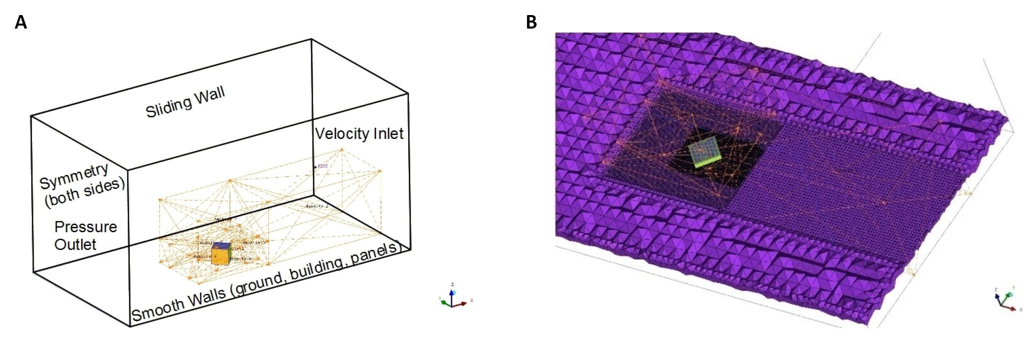
Figure 4. CFD model. A: Boundary conditions; B: Fluid mesh.

 

3 RESULTS

3.1 Force Balance Tests Configuration 3A to 10A

The results presented here are averaged on all velocities, with values of 20, 30, 40, 50, 60 (m/s). The mean pressure coefficients over the pressure taps on the roof ranged from -1.12≤Cproof≤-0.81. In the center zone where the panel is located, pressure taps (26, 27, 28, 29) monitor values in the range of -1.12≤Cppanel≤-0.84, which almost represents all the values over the roof. In this precise case, the whole roof zone is a separated zone, with no reattachment. This is mostly due to the short dimension of the roof in the along-wind direction and also because the velocity profile is not an atmospheric boundary layer type profile. The force coefficients for the configuration A tests are given in Table 1 below. Red wool threads were taped to the surface of the cube to indicate the direction of the flow; they can show the recirculating flow against the mean wind flow.

 

Table 1. Force Coefficients Measured with a Force Balance on a Single Panel

 

3.1.1 3A

Panel 20mm×120mm, 20° facing the wind: the x-component is significant and directed against the mean wind. This shows that drag is also a consideration in the design process.

 

3.1.2 4A

Panel 20mm×120mm, 20° back to the wind: In this case, the data were too sparse to be represented by a mean value. The load direction oscillates between upward and downward. Indeed, the averaged value of CFz on all velocities is not representative. On the other hand, the lift force coefficient is not significant in this configuration.

 

3.1.3 5A

Panel 20mm×120mm, 20° along the wind: this configuration is the safest for the panel as the wind does not impinge directly on the lower surface. In this case, the lift force is mostly due to pressure equalization.

 

3.1.4 7A

Panel 20mm×120mm, 20° facing the wind sheltered between two panels: The sheltering effect is evident through reduced lift and drag, nearly half compared to configuration 3A.

 

3.1.5 8A

Panel 20mm×120mm, 20° back to the wind sheltered between two panels: Fx is always positive, indicating that the force is directed against the mean wind direction. Compared with configuration 4A, the shelter effect is witnessed through reduced Fx (factor of nearly two) and a vertical force directed downwards. The recirculating flow is evident from the panel’s lower edge to the upper edge, as indicated by the red wool threads.

 

3.1.6 9A

Panel 40mm×40mm, 20° facing the wind sheltered between two panels: compared with configuration 7A, the y and z components are greater in this configuration. This confirms the influence of the panel span on the loads; a larger span tends to reduce the overall load coefficient by averaging.

 

3.1.7 10A

Panel 40mm×40mm, 20° back to the wind sheltered between two panels: in this case, the load is very small, not only due to the shelter effect but mostly because the recirculating flow is not impinging on the panel’s lower face. The large dispersion can be attributed to the balance not being calibrated to measure such small forces.

 

3.2 Wind Tunnel Tests Configuration C

3.2.1 Configuration 4C Building at 45°, Panels Facing the Wind, Lift Coefficients Averaged on All Velocities

Skewed flow cases are the most interesting configurations because of the presence of corner vortices. Moreover, the wind is more likely to form a non-zero angle with the normal direction. Wool threads showed that the flow over the roof is highly unsteady and more complex than in normal flow cases. Some zones exhibit velocities along the mean wind direction, while other zones have velocities against it. As shown in Figure 5A, pressure taps display strong downward loads as well as robust lift coefficients. If the downward load reaches a high value, the increase in contact pressure on the roof could eventually be a threat to the structure.

 

The mean values interval is -1.03 to 0.37. A relatively small dispersion over tap 23 (front row 0.37/0.51) shows that high local lift is likely to occur. Despite the local lift indicated by some pressure taps, when averaging over a panel, the tendency is toward a downward load. Indeed, the majority of the pressure taps indicate a downward load, and several indicate strictly upward loads. Taps 2, 3, 23, and arguably 9, located inside the conical vortex, monitor mean upward load coefficients of 0.089, 0.073, 0.367, and 0.103. The flow over the roof is composed of different zones; at their respective boundaries, those zones can retract (collapse) or extend (reform), which explains the fluctuating load direction on several taps. Taps 10, 13, 16, 19, 26 clearly show the boundary of the conical vortex zone. Taps in the center zone monitor mostly downward load, indicating that in the center zone, the flow is in the along-wind direction. Tap 22 monitors downward load, indicating that the flow is attached at the upwind corner. Tap 1 oscillates between upward and downward load, showing the beginning of a conical vortex.

 

Figure 5. Building at 45° lift coefficients averaged on all velocities. A: Panels facing the wind; B: Panels back to the wind.

 

3.2.2 Configuration 5C Building at 45°, Panels Back to the Wind, Lift Coefficients Averaged on All Velocities

Lift coefficients vary with the incoming velocity. However, the data does not show a clear pattern between the velocity and the lift coefficient. Low dispersion averages can be used to estimate the wind lift action; tap 15 yields the maximum lift coefficient, and dispersion is relatively small in comparison with other taps. As shown in Figure 5B, taps 1 and 22 are located on the downwind panel and monitor a high lift coefficient with low dispersion. Tap 4, which is located one panel upwind, monitors a very high lift coefficient. Taps 15, 18, and 21 are located upwind on the opposite side and monitor high lift coefficients. Tap 17, 20, 27, and 28 show high downward load coefficients. This is due to wind recirculating in the conical vortex and hence flowing on the panel from downward to upward edge. The pressure coefficient on the roof below the upwind panel takes the most negative values (-1.3 averaged), showing that the actual lift on the panel cannot be determined knowing only the pressure coefficients on the roof surface. Indeed, taps 1 and 4 have relatively low roof pressure (-0.7 averaged) coefficients. Taps 3, 6, and 9 located downwind show very weak load coefficients. Taps 10, 13, and 16 show weak load coefficients, probably because of sheltering by the upwind edge conical vortex. Tap 9 and 6 also monitor a low lift coefficient. Tap 29 shows that panels with aerodynamic protection (back and side plates) are still subject to lift. Indeed, at tap 29, we can assume that the local flow is directed along the wind and strikes on the backplate. In conclusion, skewed wind flow can be considered a threat to the panels even when those are shielded. From these results, it is obvious that panels should be mounted together in rows to average the load.

 

3.3 CFD Model Validation

3.3.1 Force Balance Tests

Table 2 shows the comparison results between wind tunnel data and CFD modelling for configuration A (force balance tests). The main discrepancy lies in the drag and drift forces, which are underestimated in CFD computations. The error in the lift force is approximately 10% which is considered satisfactory.

 

Table 2. Panel Pitch 20⁰, Comparison between CFD Computations and Wt Tests

 

Figure 6 shows the CFD model results for validation with configuration A. Pressure coefficients over the roof were more negative (indicating higher suctions) during the wind tunnel tests. These coefficients are overly negative compared to an actual building in a wind flow. This discrepancy is attributed to the blockage in the wind tunnel. Results indicate that the upper face of the panel has a slightly more negative pressure coefficient than the roof right below, resulting in a lift force exerted on the panel.

 

Figure 6. Velocity vectors at mid-plane around the panels. A: Configuration 1, contours of Cp30.35; B: Configuration 7, contours of Cp30.75.

 

3.3.2 Solar Panel Array with Aerodynamic Protection; Cube at 45°, Panels Back to the Wind (Wind Tunnel Tests Configuration 5c)

In the wind tunnel tests for Configuration 5C, the panels faced back to the wind, and the lift coefficients observed were higher. It was deemed more relevant to validate the model using the worst-case scenario among the various tested configurations. The simulation settings included a constant wind velocity at the inlet boundary set at 19.6m/s. The results revealed that achieving complete agreement between tap (WT) and tap (CFD) was challenging. Only partial agreement was observed, with some taps showing good or fair agreement while others diverged. However, when pressure taps are put together for each panel, as shown in Table 3, and their values are averaged accordingly, better agreement could be reached.

 

Table 3. Lift Coefficients, Configuration 5c, Comparison Between Cfd and Wt

 

Discrepancies between the wind tunnel tests and CFD simulations arise from differences in the flow structure over the roof. In the wind tunnel tests, the pressure coefficient was strongly negative over the entire roof due to blockage. In the CFD computations, both strong negative coefficients (indicating separation zones) and weak negative coefficients (indicating attached flow zones) were observed. Table 3 shows that discrepancies are mainly evident for the upwind panels situated in the conical vortex zone. For these panels, CFD computations yield more conservative mean load coefficients when designing for wind loads. Consequently, the present CFD model is considered capable of assessing wind loads on rooftop solar panels.

 

3.4 Wind Loads on the Rooftop Solar Panel Array in Design Wind Conditions

3.4.1 Boundary Conditions

In this scenario, the flow pattern aims to emulate design wind conditions. The velocity profile at the inlet adheres to the SIA 261 norm (Swiss norm), representing a 50-year return period maximum gust pressure. Hence, it signifies the maximum wind velocity anticipated during the panels’ lifespan. According to the norm, the design wind speed at roof height is specified as Vdes=38m/s. In this particular design case, there are no available measurements for validating the CFD model. However, pressure coefficients for cubic structures are well-documented[24], providing a reliable reference for assessing the model's accuracy. The pressure coefficients on the building envelope are calculated as per the following equation:

 

 

Certainly, a precise evaluation involves a comparison between the computed pressure coefficients over the building envelope and reference values. This comparative analysis allows us to determine if the simulated flow aligns with an actual wind flow. In this context, the reliability of the wind loads information provided by the CFD model for design purposes can be established. Figure 7A illustrates the lines a-b, b-c, and c-d, where the evolution of pressure coefficients is monitored, and these lines are located at the midplane. For each configuration, the pressure coefficients along these lines must align with the reference pressure coefficients available in wind codes.

 

Figure 7. Wind loads in design wind conditions. A: Orientation of the cubic building; B: Inlet velocity profile.

 

Moreover, we consider the incorporation of aerodynamic protection or a shielding backplate. The panels are modeled as interconnected pitched flat plates (walls) with zero thickness. Consequently, a single lift coefficient is assigned to each panel. The computation of design pressure coefficients (positive upwards) on the solar panels follows the formula:

 

 

3.4.2 Wind Coming at 45° from the Windward Face, Panels Back to the Wind

It is well-documented that pressure coefficients over the roof are the most negative for wind angles between 30° to 45° when conical vortices are the strongest. Present computations showed that the conical vortices have Cp38 values between -2.5 and -1.5. Extremely negative pressure coefficients occur locally at the corners with values ranging from -3 to -4.5. When plotting the pathlines in the mid-plan, we notice that the wind smoothly flows around the cube. Fewer streamlines flow over the cube compared to the normal flow situation. As shown in Figure 8, except for the conical vortices, there is no significant separation bubble. We notice that the flow is attached to the roof; pressure coefficients along the roof mid-line rapidly take a lower suction value, indicating attached flow. The higher lift force on the panels in this case is due to the fact that the incoming wind impinges directly on the lower face of the panels.

 

Figure 8. Design wind incoming at 45°. A: Velocity vectors (m/s) above the panels and pathlines from the windward edges (colored by ID) computed lift coefficients Cdes (positive upwards); B: Without shielding backplate; C: With backplate.

 

The first row of panels experiences a downward force, which aligns with the findings from configuration 5C in the wind tunnel tests. Due to the delta-wing vortices, the flow on the front row is oriented along the panels (parallel to the windward edge) and not crosswise, generating no lift force on the panels but rather a downward force. Lift occurs precisely when the flow is crosswise and impinging on the lower face of the panels. Some panels experience high lift coefficients, particularly those located on the +x side. The corner vortices determine three distinct flow regions, as shown in Figure 8A: two conical vortices with recirculating flow and an attached flow region. Moreover, Figure 8B and 8C show that lift coefficients are very high in the attached flow zone and low or negative elsewhere. This is precisely where shielding using a backplate makes sense. Except for several panels, border zones are not critical. This shows the irrelevance of building codes for rooftop solar panels; the border zones are critical for the roof envelope itself, but the pressure difference across the panels in those zones is not of similar magnitude. The influence of backplates to reduce lift by shielding the wind is straightforward, as we witness an overall significant lift reduction. In the two configurations, there is a significant difference between the load on the front row of panels.

 

3.4.3 Wind Coming Normal to the Windward Face, Panels Facing the Wind

This case is significant as it illustrates the impact of the building-induced flow disturbance on the lift coefficients of the panels. The vorticity initiated at the windward edge results in a high lift force on the panels. As shown in Figure 9, in the separation bubble, the wind is recirculating and impinging on the lower face of the panels. Plotting pressure coefficient isosurfaces in Figure 9C reveals a substantial separation bubble (Cp38=-0.5) encompassing almost the entire building. The zone from the separating edge, including the first panel, is within a bubble with Cp38 values ranging between -1.5 and -1. Pathlines show that the entire roof is in a separated zone, with no reattachment. Additionally, Pathlines reveal the presence of a horseshoe vortex at the windward face near the ground. Lift coefficients decrease from row to row, reaching maximum values at the windward edge and minimum values at the leeward edge. Lift is primarily due to the recirculating flow impinging on the panels’ lower face. Once again, shielding the panels would contribute to reducing the lift force.

 

Figure 9. Design wind incoming at 90°. A: Velocity vectors at plane y=0 colored by velocity magnitude (m/s); B: Computed lift coefficients Cdes; C: Contours of pressure coefficient Cp38 together with pathlines colored by ID and isosurface Cp38= -0.5.

 

3.4.4 Wind Skewed at 30°, Panels Facing the Wind

In this configuration, illustrated in Figure 10A, the overall trend is towards a downward force. Nevertheless, there are still instances of high lift coefficients, especially on the first row (windward row) of panels, predominantly experiencing lift due to the recirculating flow. The highest computed lift coefficient reached 0.48 on a single panel. The panels situated within the zone delimited by the conical vortex, as shown in Figure 8A, experience lift. However, other panels within the attached flow zone experience a downward force. In this particular configuration, the implementation of a shielding backplate wouldn't contribute significantly.

 

3.4.5 Wind Skewed at 15°, Panels Back to the Wind

In this configuration, depicted in Figure 10B, notable lift coefficients are observed near the +y leeward corner and along the +y edge. This lift is attributed to the attached wind flowing across the panels and impinging on their lower faces. This particular zone appears more susceptible, highlighting the necessity of introducing shielding backplates and averaging the load with panels in the center. Among all the simulated configurations, this scenario yielded the maximum lift coefficient, reaching 0.59. The majority of the panels experience either a downward load or weak lift due to the recirculating flow within the expansive conical vortex region.

 

Figure 10. Computed lift coefficients Cdes. A: wind at 30° panels facing the wind; B: wind at 15° panels back to the wind.

 

4 DISCUSSION AND CONCLUSION

Wind engineering design coefficients typically applicable to bare roofs are not directly transferable to rooftop elements like solar panels. The wind load on rooftop elements comes from the pressure difference between the upper and lower faces, a factor primarily influenced by the local velocity direction and intensity. The local flow pattern is significantly affected by parameters such as the building’s orientation in the incoming wind (building flow field), panel geometry and arrangement, building geometry, and turbulence intensity. Over the past two decades, various studies employing full-scale measurements and BLWT testing have sought to enhance the accuracy of lift coefficients for updating standard design guidelines. In the present study, both wind tunnel tests and CFD modeling were conducted. The validity of the CFD model was assessed not only by comparing it with the experimental data from this study but also by comparing the computed roof pressure coefficients with reference values. The CFD model provided design pressure coefficients for multiple wind directions. The wind tunnel tests revealed that, within the separation bubble, the load on the panels is predominantly influenced by the wind direction and to a lesser extent by the panel geometry and pitch angle. Moreover, the shelter effect within the array acted to locally reduce the loads. It is crucial to note that wind load is a local quantity, and the practice of averaging over large zones may not be a reliable approach. Upward and downward loads can occur simultaneously at different locations within the array.

 

In conclusion, the study yields the following key observations:

(1) Within the conical vortex zone or separation bubble: higher lift force coefficients are due to the pressure equalization together with the recirculating flow impinging on the lower surface of the panels. Design considerations should prioritize addressing the challenges posed by the conical vortex, with computed lift coefficients reaching as high as 0.7.

(2) Among the attached flow region: higher lift force coefficients in this region result from the wind directly impacting the lower face of the panels. When the wind impinges on the upper face (from lower edge to upper edge), downward load occurs.

(3) When the flow is directed along the span of the panels, it generates no significant load or downward force.

(4) The shielding backplate is very effective at reducing lift when the wind would impinge on the lower face of the panels instead.

 

The most practical strategy to mitigate loads involve introducing porosity to the system for controlled pressure equalization between the lower and upper surfaces of the panels. Additionally, mounting panels together in rows facilitates load averaging, offering protection against lift-off, with the added benefit of addressing potential concerns related to drag.

 

The most accurate method for determining lift coefficients at a specific site involves placing load cells on the actual rooftop panels’ supporting frame while concurrently measuring the mean incoming wind speed and direction. This approach is particularly justified for large-scale installations with significant investment costs, providing real-world, site-specific data. In cases where on-site measurements are not feasible or are cost-prohibitive, wind tunnel studies and CFD modeling become valuable tools. These methods offer more accurate and design-specific information compared to relying solely on coefficients from generic wind codes. The values in wind codes may often be either overestimated or not directly applicable to the unique.

 

Acknowledgements

Many thanks to Christophe Cerutti for his help in building the model used in the wind tunnel tests.

 

Conflicts of Interest

The authors declared no conflict of interest.

 

Author Contribution

Haas P and Binyet E designed the experiment, Haas P supervised the work. Binyet E performed the data analysis. Binyet E drafted the manuscript. All the authors contributed to writing the article, read and approved its submission.

 

Abbreviation List

CFD, Computational fluid dynamics

PV, Photovoltaic

 

References

[1] Aziz AS, Tajuddin MFN, Zidane TEK et al. Design and Optimization of a Grid-Connected Solar Energy System: Study in Iraq. Sustainability, 2022; 14: 8121.[DOI]

[2] Tran TS, Vu MP, Pham MH et al. Study on the impact of rooftop solar power systems on the low voltage distribution power grid: A case study in Ha Tinh province, Vietnam. Energy Rep, 2023; 10: 1151-1160.[DOI]

[3] Khairi NHM, Akimoto Y, Okajima K. Suitability of rooftop solar photovoltaic at educational building towards energy sustainability in Malaysia. Sustainable Horizons, 2022; 4: 100032.[DOI]

[4] Chakraborty S, Sadhu PK, Pal N. Technical mapping of solar PV for ISM‐an approach toward green campus. Energy Sci Eng, 2015; 3: 196-206.[DOI]

[5] American Society of Civil Engineers. Minimum Design Loads and Associated Criteria for Buildings and Other Structures. ASCE/SEI 7-16. ASCE: Washington. USA, 2017.

[6] Japanese Standards Association. Load design guide on structures for photovoltaic array. JIS C: Tokyo, Japan, 2017.

[7] Radu A, Axinte E, Theohari C. Steady wind pressures on solar collectors on flat-roofed buildings. J Wind Eng Ind Aerod, 1986; 23: 249-258.[DOI]

[8] Ruscheweyh H, Windhövel R. Wind loads at solar and photovoltaic modules for large plants: Proceedings of the 13th International Conference on Wind Engineering. Amsterdam, The Netherlands, July 2011.

[9] Kray T, Hunke F. Windlasten an den PV-Flachdachsystemen DuoFlat und DuoFlat DS der Palme Solar GmbH Bestimmung der abhebenden und verschiebenden Lastkennwerte. Institut für Industrieaerodynamik GmbH Institut an der Fachhochschule Aachen, 2012.

[10] Geurts CPW, van Bentum C, Blackmore P. Wind loads on solar energy systems, mounted on flat roofs. EACWE 4, 2005; 124.

[11] Geurts CPW, van Bentum CA. Local wind loads on roof-mounted solar energy systems. Recent advances in research on environmental effects on buildings and people. 2010; 195-206.

[12] Pratt RN, Kopp GA. Velocity measurements around low-profile, tilted, solar arrays mounted on large flat roofs, for wall normal wind directions. J Wind Eng Ind Aerod, 2013; 123: 226-238.[DOI]

[13] Stathopoulos T, Zisis I, Xypnitou E. Local and overall wind pressure and force coefficients for solar panels, J Wind Eng Ind Aerod, 2014; 125: 195-206.[DOI]

[14] Banks D. The role of corner vortices in dictating peak wind loads on tilted flat solar panels mounted on large, flat roofs. J Wind Eng Ind Aerod, 2013; 123: 192-201.[DOI]

[15] Banks D. The suction induced by conical vortices on low-rise buildings with flat roofs. Colorado State University: Fort Collins, USA, 2000.

[16] Cao J, Yoshida A, Saha PK et al. Wind loading characteristics of solar arrays mounted on flat roofs, J Wind Eng Ind Aerod, 2013; 123: 214-225.[DOI]

[17] Kopp GA, Farquhar S, Morrison MJ. Aerodynamic mechanisms for wind loads on tilted, roof-mounted, solar arrays, J Wind Eng Ind Aerod, 2012; 111: 40-52.[DOI]

[18] Bienkiewicz B, Endo M. Wind considerations for loose-laid and photovoltaic roofing systems: Proceedings of the Structures Congress 2009: Don't Mess with Structural Engineers: Expanding Our Role. Austin, Texas, April 30-May 2 2009.[DOI]

[19] Naeiji A, Raji F, Zisis I. Wind loads on residential scale rooftop photovoltaic panels, J Wind Eng Ind Aerod, 2017; 168: 228-246.[DOI]

[20] Estephan J, Chowdhury AG, Irwin P. A new experimental-numerical approach to estimate peak wind loads on roof-mounted photovoltaic systems by incorporating inflow turbulence and dynamic effects. Eng Struct, 2022; 252: 113739.[DOI]

[21] Bender W, Waytuck D, Wang S et al. In situ measurement of wind pressure kloadings on pedestal style rooftop photovoltaic panels. Eng Struct, 2018; 163: 281-293.[DOI]

[22] Chung PH, Chou CC, Yang RY et al. Wind Loads on a PV Array. Appl Sci, 2019; 9: 2466.[DOI]

[23] Fluent A. ANSYS Fluent Theory guide 15.0. ANSYS, Canonsburg PA, 2013. 33

[24] Richards PJ, Hoxey RP, Connell BD et al. Wind-tunnel modelling of the Silsoe Cube. J Wind Eng Ind Aerod, 2007; 95: 1384-1399.[DOI]

 

Copyright © 2023 The Author(s). This open-access article is licensed under a Creative Commons Attribution 4.0 International License (https://creativecommons.org/licenses/by/4.0), which permits unrestricted use, sharing, adaptation, distribution, and reproduction in any medium, provided the original work is properly cited.