Origins of "Natural Climatic Nervousness" and its Current Accentuation

 

Éric Zeltz1*

 

1Independent Researcher, La Motte en Champsaur, Hautes-Alpes, France

 

*Correspondence to: Éric Zeltz, PhD, Professor, No Affiliation (Independent Researcher), 5 route du Moulin, La Motte en Champsaur, Hautes-Alpes 05500, France; Email: ericzeltz@wanadoo.fr

 

DOI: 10.53964/jmge.2023008

 

Abstract

Objective: We would like to give the climatological explanations of two probabilistic observations made from temperature data analyzed in a 2021 article: (1) The time series made up of the monthly "increases" in the average global temperature for the period 1880-2014 calculated from a database provided by the American agency National Oceanic and Atmospheric Administration has the behavior of a Markov chain of order 1, in particular insofar as if a positive increase is observed (in other words an increase in temperature compared to the month which precedes) such a month, the probability is stronger that it will be negative the following month, and vice- poured. (2) This "forced" alternation, a phenomenon that we will designate in this work by the expression "natural climatic nervousness", accelerated considerably from the 1970s.

 

Methods: From the time series at play, we detect "signals" that allow us to highlight possible interactions capable of explaining them. To validate these explanations, we are developing a simple climatological model to verify that the proposed explanations are well integrated.

 

Results: We show that the origin of this phenomenon is certainly an interaction of the heat of the Troposphere with that from the upper ocean layer, through the evaporation that occurs at the surface of the oceans. Then we develop a discrete modeling of the oceans / troposphere coupling which, although rudimentary, makes it possible to a certain extent to confirm our hypothesis on the anticipated origin of this "natural climatic nervousness". The particular phenomenon of acceleration of the natural climatic nervousness observed since the 1970s is explained in a coherent way with the general phenomenon, that by using an observation of the increase in the stratification of the upper oceanic layer.

 

Conclusion: This article shows the interest of the method which is used there, both simple to implement and effective in obtaining interesting results which would undoubtedly be much more difficult to obtain with more traditional methods. Similarly, the interest of the discrete model of the ocean / troposphere coupling developed with the aim of verifying the correct integration of the explanations obtained in the evolution of the climate appears clearly: it is both realistic in the simulations it generates and technologically much more accessible for its implementation than the global climate models developed and used by the main climatological institutes.

 

Keywords: climate change, climate modeling, time series, Markov chains, evaporation, dynamic heat capacity

 

1 INTRODUCTION

The importance for climate and the complexity of the ocean-atmosphere interaction have long been known[1-4]: the role of ambient water vapor and clouds[1,2], the response of atmospheric winds to the temperature of the upper ocean layer and its gradient[3], its influence on extreme rainfall events[4], the selective absorption of radiation by the ocean[1], the distribution of total warming in the ocean-atmosphere system[1], etc., all these phenomena interact with each other in complex ways and anything that advances their understanding helps to reduce the uncertainties in the simulations provided by global climate models.

 

It is in particular for this last purpose that we introduce here a new method whose results will allow us to move forward an interesting way to understand this interaction at the level of the planet.

 

In order to allow a simplified access to it, let us start by suggesting a reflection about a situation in probability which will be very often present in this article and which is the key to this method:

 

Suppose we have a well-balanced coin, so with the same probability of 0.5 of falling heads (denoted H) as tails (denoted T). We toss this coin a hundred times and note each successive occurrence. There is a tiny probability of (½)100, or less than one chance in a billion billion billion, that we have a constant alternation like HTHTHTHT…HTHT. In fact, this situation is governed by a binomial law with parameters P=0.5 and n=100 for which we know that the chains of successive H (same thing for the T) are, in terms of mathematical expectation, distributed according to this Table 1 (page 42 of Delmas[5]):

 

Table 1. Theoretical Frequencies Relative to the Total Number of Strings of a Substring of H (or T) of a Certain Length for Series of One Hundred Throws

 

Now back to our streak of one hundred throws. The experiment ended, we realize that in fact the average length of the chains of successive P is clearly lower than the theoretical figure of 1.94, that there are many more chains of 1 and 2 than the frequencies predict, and much less for chains of 3 and more. So the alternation is much faster than predicted by theory. It can happen, and at this point there is no reason to question the truly binomial character of the experiment.

 

On the other hand, if we redo this experience of a hundred throws 10 times in a row, and each time we find this alternation clearly accelerated, we have to ask ourselves questions: it is almost impossible that this is only the result of chance, and the coin itself is not in question since it is perfectly balanced. So there is most certainly an interaction of the throws with an external phenomenon. From what origin does this interaction come - phenomenon of periodic electromagnetism or others? - we cannot specify this without first carrying out an additional investigation, but we can affirm with practically no risk of being mistaken that there is indeed an interaction with an external phenomenon. This constant average length less than the theoretical length of the successive P chains is therefore the "signal" of a certain interaction.

 

As we present in Table 2 whose data is taken from Zeltz[6], it is exactly this situation that has been noted concerning the rises in global average monthly temperatures over the period 1880-2015: for the 16 hundreds of monthly occurrences concerned, each having a probability very close to 0.5 for a rise or fall as verified, it was found that each of these series has always its average lengths of rise chains lower than the theoretical average of 1.94. Climatological situation that we will therefore designate by the expression "natural climatic nervousness". Moreover, we observe a notable acceleration of this phenomenon for the last five series marked with an asterisk which correspond to the period 1970-2015.

 

Table 2. Average Lengths of the Rise Chains for the Sixteen Sequences of One Hundred Temperature Anomalies from the Period 1880-2015

Notes: *, notable acceleration period 1970-2015 marked with an asterisk; Data Source: Zeltz[6]

 

Assuming that all of this is governed by the binomial distribution B100 with parameters P=0.5 and n=100, the probability of such a situation is already very low: (½)16, i.e. of the order of a chance out of sixty five thousand. But still on the assumption of the binomial law B100, if we refine the calculation by taking into account that eleven of the sixteen average lengths in question are less than 1.7, three between 1.7 and 1.85, and only two very close to the theoretical average (1.91 and 1.92 instead of 1.94), this leads to a probability of less than one chance in a billion! As for the post-1970 period of acceleration of this natural climatic nervousness, where the average lengths of the five series of hundred concerned do not exceed 1.64 and are very often closer to 1.40, the probability of having such a situation governed by law B100 would be far less than a one in a hundred million chance! So of course, we cannot completely exclude that this very specific phenomenon is the consequence of some bias in the implementation of the database concerned and coming from NOAA, but what bias knowing that this institute is renowned for the reliability of its climatological databases?

 

As illustrated by our example of coin tossing, the presence of a second climatological actor capable of interacting with the global average monthly atmospheric temperature, namely the upper ocean layer, therefore seems to us essential. We show that the hypothesis resists very well to the analysis of the climatological series concerned, the "signals" carried by the time series in question being consistent with this explanation. It therefore seemed important to us to devote a paragraph intended to take stock of our method, to specify its advantages but also its inherent limits.

 

Following these, additional checks must therefore be made by more conventional methods or using simulations.

 

This is the main reason why, in a whole important section entirely dedicated to this, we set up a climatological model: the simulations that we will obtain through it will allow to a certain extent to validate our explanation by showing that it does not does not contradict the results from these simulations. Moreover, we can see that this model is of great interest by itself. In particular, it seems to us that non-specialists in climatology equipped with a minimum of scientific culture will be able thanks to it to truly grasp the reality of climate change, much better than by the almost blind confidence that they owe for the instant give to the results appearing in the reports of the major climatological institutes.

 

Finally, concerning the acceleration of natural climatic nervousness observed from 1970, we propose an explanation consistent with that of the general phenomenon.

 

2 MATERIALS AND METHODS

2.1 Presentation of the Data and Details on the Probabilistic Choices Made

Table 3 presents the two types of climate anomaly data involved in this article:

 

Table 3. Description of the Data Studied

 

The first series is almost the same than the one that was used in Zeltz[6] and from which the data in Table 2 is taken, with the only difference that it stops in 2022 instead of 2015.

 

The climatic entities which correspond to these two series are dependent on highly non-linear evolutions, therefore without any apparent influence of what may have happened for them a few weeks before, letalone a few months (Lorenz[7], Le Treut and Jancovici[8]). This is part of what climatologists call phenomena with weak climatic memory, meaning having the property to "forget" quickly their initial conditions.

 

For atmospheric phenomena such as the average temperature on the ground, precise forecasts concerning them do not exceed ten days, and this still identifiable climatic memory is of the order of a month (Shukla[9], Pailleux[10], Buizza and Leutbecher[11]), which therefore corresponds to the periods of the time series concerning them.

 

For ocean heat, subject to significant thermal inertia, the climatic memory is greater, on the order of two or three months (Stock et al.[12], Shi et al.[13]). Again, a duration fairly close to that of the periods of the time series studied which concern it.

 

Let (Xk) be any one of these two time series. Let then (Yk=Xk-Xk-1) be the time series derived from the "deviations" associated with (Xk), and finally let (Mk) be the series formed solely of 0 and 1, where 0 corresponds to a negative deviation (a decrease for Xk) and 1 to a positive deviation (an increase for Xk). The first step of our analysis consisted in verifying that (Yk) is stationary in the weak sense (Hamilton[14], page 45 for the definition and page 682 as a property of Markov chains). Then, taking into account the climatic memory of the phenomena involved, the only probabilistic schemes which then seem possible to us and really suitable for modeling (Mk) are Markov chains of order 1 (Markov chains in the strict sense), or those of order 0 (thus here simple binomial laws). To decide between these alternatives, it is the frequencies and average lengths of the "ascent chains" (formed exclusively of 1) and those of the "descent chains" (formed only of 0) which provide us with a "signal" allowing us to choose between the three a priori possible situations: chain governed by a binomial law (terminology used subsequently: binomial Markov-0 signal), Markov chain of order 1 of the "lengthening" type (lengthening Markov-1 signal), and finally chain of order 1 of the "alternating" type (alternating Markov-1 signal).

 

Indeed, as we specified in our introduction, the binomial laws have statistically a distribution and an average length of their very characteristic chains of rise or fall, which will therefore be different from those of the Markov chains of order 1 ( Delmas[5]).

 

2.2 Other Justifications

For many points, our approach is quite different from that which is classically used in climatology, so here we will comment and justify some of the positions adopted in this work and compare them to the more classical choices usually made in climatology:

(1) The data studied is global data, and therefore, whatever the month or quarter considered, all the seasons are represented there on the surface of the globe and are therefore included in the calculation of these averages. In fact, the question of seasonal adjustment does not arise for this type of data. This means that, for example, when NOAA chooses January as the reference month to establish its global atmospheric temperature anomalies, it could have chosen any other month of the year in an equivalent manner.

 

(2) Throughout the period 1955-2022 of our study, the climate has undergone numerous disturbances with significant repercussions on a global scale. This period, for example, has experienced many intense El Niños[15] episodes and episodes of La Niña, the first leading to global warming and the second to cooling. (Kim and Cai[16]). Other events with significant climatic repercussions, the eruption of El Chichón in 1982 and that of Pinatubo in 1991, in particular because of the considerable masses of particles that they emitted into the atmosphere. For example, the Pinatubo eruption caused global cooling over nearly two years (Self et al.[17]). Also noteworthy is the concentration of aerosols of anthropogenic origin in the atmosphere, which changed a great deal during this period, in particular due to the dissolution of the USSR and what it entailed for the economies of the countries of the Eastern Europe (Cherian et al.[18]). And this concentration has many influences on cloud formation and global temperature (Nabat et al.[19]). However, we have chosen not to filter our numerical series to eliminate the disturbances brought by all these phenomena. This position is justified by the fact that we only work on the sign of the differences (translated by a 0 in the event of a descent, a 1 in the event of an ascent) between two successive anomalies. This deliberate choice, although it results in a large loss of information in the processed data, has the advantage of making it possible to obtain in a very simple way interesting "signals" which are much less disturbed by the phenomena of the preceding type than are the initial raw data. As proof of this, we have found that for the three series considered, the probabilities of a rise or fall are always very close to 0.5, even when we place ourselves on sub-periods oriented towards an increase, or even towards a decline, or finally rather stable.

 

(3) Similarly, phenomena as important as atmospheric winds or ocean currents are not specifically taken into account in the analysis of the signals. And when it comes to developing an ocean / troposphere climate model, they will indeed, but in a very rudimentary way, thanks to the use of a concept of "dynamic heat capacity" introduced on this occasion. As we will see, this will be enough to obtain completely realistic simulations.

 

(4) The rest of what constitutes the "natural variability" of the climate will be taken into account by introducing random coefficients into the model.

 

2.3 Comparison of the Evolution of the Surface Thermal Energy of the Oceans with that of the Global Average Temperature Over the Period 1955-2022

Concerning the heat (i.e. thermal energy) anomalies in the upper layer of the oceans (between 0 and -700m), it is still the NOAA which provided us with the data (link in Table 3). These anomalies were calculated relative to the average for the period 1955-2006 and are given quarterly from the beginning of 1955 to the end of 2022, a unit corresponding to 1022 joules. We put them into perspective with the quarterly temperature anomalies, obtained from the monthly global temperature averages provided by NOAA for the same period (link in Table 3). They will still be expressed in tenths of a degree Celsius. In order for the zero to correspond to the average state over 1955-2022 for each of these two series, we subtracted their respective average over the period 1955-2022. Figure 1 presents the curves thus obtained accompanied by the associated linear regression lines.

 

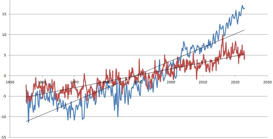
Figure 1. Comparative evolution of the two types of anomalies. Red curve: Quarterly atmospheric temperature anomalies in tenths of °C; Blue curve: Quarterly heat anomalies in the upper ocean layer, 1 unit =1022J; Period considered: 1955-2022; Source: NOAA.

 

The good correlation between the two series is confirmed by its coefficient since it is equal to 0.85.

The rates of these increases are as follows:

- about 0.1°C per decade for atmospheric temperature.

- 3.3×1022J approximately per decade for the ocean heat present in the upper layer of the oceans.

 

We then looked at the distribution according to their length of the chains of ascents and descents. Indeed, the comparison with the theoretical results (expectations) expected for a binomial law Bn (n; P=0.5) will allow us to determine the underlying probabilistic model: binomial Markov-0, Markov-1 alternating or lengthening Markov-1.

 

For this, it will just require to compare the distributions according to their size of the chains of climbs and descents, as well as their average lengths, with the theoretical frequencies (mathematical expectations) obtained for a Markov chain made up of 0s and 1s and subject to this binomial distribution Bn (n; P=0.5) and which are specified in Table 1 of our introduction for the case of n=100.

 

Given the number of quarters at play (270=3×90) and the number of months at play (one little more than 800=8×100) over the period 1955-2022 of the study, we will consider two values of n: n=90 and n=100. But as we were able to verify, the passage of B100 at B90 practically does not modify the distributions according to the size of the chains nor their average length as given in Table 1 for the case of law B100.

 

The results are collected in Tables 4-6.

 

We highlight with an asterisk the average lengths clearly below the length average of a chain governed by the binomial distribution at play (1.94), without an asterisk those which are very neighbors (in the range [1.80; 2.10]), with two asterisk those which are clearly superior.

 

Table 4. Average Frequencies of Occurrence by Length and Average Lengths of Chains of Ascents and Descents of Ocean Heat Variations Present for Series of 90 Consecutive Quarters

Notes: Second to last line, similar results but for the entire period 1955-2022 studied, i.e. for 270 consecutive quarters; Last line, frequencies and theoretical average length of the chains (rise or fall) for the binomial law B90 with parameters n=90 and P=0.5; An asterisk, average length less than 1.80; two asterisk, better than 2.10.

 

Table 5. Average Frequencies of Occurrence by Length and Average Lengths of Chains of Ascents and Descents of Atmospheric Temperature Differences Present for Series of 100 Consecutive Months

Notes: Second to last line, Similar results but for the entire period 1955-2022 studied, i.e. for 816 consecutive months; Last line, Frequencies and theoretical average length of the chains (rise or fall) for the binomial law B100 with parameters n=100 and P=0.5; An asterisk, average length less than 1.80; two asterisk, better than 2.10.

 

Table 6. Average Frequencies of Occurrence by Length and Average Lengths of Chains of Ascents and Descents of Atmospheric Temperature Differences Present for Series of 90 Consecutive Quarters

Notes: Second to last line, similar results but for the entire period 1955-2022 studied, i.e. for 270 consecutive quarters; Last line, frequencies and theoretical average length of the chains (rise or fall) for the binomial law B90 with parameters n=90 and P=0.5; An asterisk, average length less than 1.80; two asterisk, better than 2.10.

 

Here are our main observations about the previous three tables:

(1) Regarding quarterly ocean heat anomalies, we are almost always in the case of alternating Markov-1 signal chains, with two exceptions where the average lengths are in the range [1.80; 2.10]. Overall, the signal is clearly of alternating Markov-1 type.

 

(2) As had already been remarked by Zeltz[6] for the entire period 1880-2015, we find an alternating Markov-1 type signal for the monthly atmospheric temperature anomalies for the period 1955-2022, with only one exception out of the sixteen series studied.

 

(3) On the other hand, with the quarterly anomalies of global atmospheric temperature, the signal carried by the series obtained is frankly of the binomial Markov-0 type, the only exception where the signal is different (of the lengthening Markov-1 type) being in fact very insufficient in order to challenge this probabilistic observation.

 

In summary:

(1) Chains with the alternating Markov-1 signal for the series of mean monthly departures from the global mean temperature.

 

(2) Chains with the alternating Markov-1 signal for the series of average quarterly deviations of the ocean heat present in the first layer (between 0 and -600m).

 

(3) Chains with the binomial Markov-0 signal for the series of mean quarterly global mean temperature deviations.

 

3 RESULTS AND DISCUSSION

3.1 Climatological Interpretations

Here are our climatological interpretations of the previous results:

(1) Let us first define what we will call the Upper Oceanic Stratum (denoted below UOS): This is the global oceanic surface layer 50 to 200m thick (Le Calvé[20]) where the temperatures are not very far from that of the surface, and located immediately above the Thermocline from which the gradient of temperature drop suddenly becomes very important. If during a month, the temperature of the Troposphere rises, the relative humidity of the air drops, and therefore the vaporization at the surface of the UOS tends to increase. This vaporization then causes a cooling of this surface of water because a important part of the calories which are necessary for it are taken within it, another part being taken in the ambient air, the ratio between the two depending above all on the difference between water and ambient air temperatures. This cooling is then propagated by conduction and convection towards the Troposphere, which explains why the probability that the atmospheric temperature dropsthe following monthis slightly greater than it rises, and this all the more so since the preceding warming has been strong. If, on the contrary, during a certain month, the temperature of the Troposphere drops, the vaporization of surface water is less easy. Thus there are fewer calories to draw from the UOS and from the ambient air to feed this evaporation which is falling and solar heating can more easily take over from the cooling caused by evaporation, whether on the surface of the UOS or just above. The following month, the probability that the temperature of the Troposphere will increase is therefore slightly higher than that of decreasing. This is how we explain this "climatic nervousness" which causes the monthly average temperature of the atmosphere to have its deviations which carry an alternating Markov-1 signal.

 

(2) As we have just seen, the surface water of the UOS interferes with the monthly cycles of the Troposphere by accentuating or on the contrary decreasing the evaporation which starts from its surface. The variations in its temperature are therefore certainly quite in phase with those of the air immediately above it, with however probably a slight shift. But for the entire UOS itself, much larger than the upper layer of water which bears the brunt of atmospheric temperature variations and cooling following evaporation, the new thermal equilibrium is much longer to obtain, in particular because of its volume and its high inertia. Ocean waters have a high thermal inertia. For example, Mediterranean waters reach their maximum temperature between one and two months after the summer peak in atmospheric temperatures (Le Calvé[20]). In addition, because of the heat capacity of water, which is four times greater than that of air, and because of the phenomenon of stratification, the UOS plays the role of the main intermediate reservoir with the rest of the ocean. a large part of the heat comes from solar radiation or that trapped by the greenhouse effect (Gettelman and Rood[21]). Indeed, more than 90% of the excess heat caused by the current energy imbalance is absorbed by the oceans (Li et al.[22]), therefore primarily by this UOS. The stratification of ocean waters largely prevents part of the mixing of these hot waters with the colder and denser lower layer formed by the thermocline and this phenomenon is accentuated with global warming[22]. One month is therefore certainly not enough to perceive something significant concerning the variations of heat and therefore of temperature on the whole of the UOS. On the other hand, a duration of three months seems sufficient since it corresponds approximately to three full cycles for the temperature of the Troposphere, and therefore a priori: Ascent, Descent, Ascent (ADA) or Descent, Ascent, Descent (DAD). This with a certain offset from the Troposphere, due to oceanic inertia. If for example for a certain quarter we are in the ADA case, there is a slightly higher probability that the UOS is in a slight rise in heat, since i there are two ascents for one descent. And the following quarter, a priori rather DAD type, a slightly higher probability that it will be downhill. And so on, quarter after quarter. In our opinion, this explains why the deviations from the quarterly averages of the upper ocean heat anomalies carry an alternating Markov-1 type signal.

 

(3) The phenomena that govern atmospheric temperatures and more generally what concerns meteorology are highly non-linear and unstable with respect to the initial conditions, therefore with an apparent rapid erasure of all memory: the atmospheric climate seems to evolve from completely independently of what it was a few weeks earlier. This phenomenon is well known and explains, for example, that meteorologists can give fairly reliable forecasts a few days or weeks after a known initial situation, but that these forecasts quickly turn into much less precise "trends" beyond three or four weeks. All the more so for longer periods where we gradually leave the field of weather forecasts to arrive at that of climatology. So, at the scale of the quarter, it seems normal that what is observed over such quarter in global atmospheric temperature does not seem to influence in one way or another what happens the following quarter, contrary to what can happen from month to month. On the other hand, as we specified in the previous point, with regard to the oceans whose heat capacity is more than a thousand times that of the atmosphere and which are affected by a much slower dynamics and an inertia very large thermal, the scale of the quarter remains largely short enough for a certain apparent climatic memory to play from one quarter to the next.

 

3.2 Update on the Method Used

There are basically three types of climatology (El Khatri[23]):

(1) Descriptive climatology which consists in describing and comparing the climates in given places or periods.

 

(2) Physical climatology which tries to highlight the physical mechanisms of atmospheric and oceanic behavior from a set of observation data.

 

(3) Dynamic climatology, which consists of finding what is revealed by observation, in particular that resulting from descriptive climatology, and projecting it into the future by a whole series of appropriate means and in particular by numerical modelling: this includes the knowledge of fluid mechanics, turbulence, energy and material transfers, physical laws governing exchanges between different environments, etc. And this leads in particular to global climate models with which simulations are obtained that feed the relationships of the Intergovernmental Panel on Climate Change.

 

Most recent articles in climatology, whether for local or global studies, obtain projections from observed data using existing models and placing themselves in various scenarios of climate change (for example: Giorgi[24], Wyant et al.[25], Meehl et al.[26]). In other words, these studies move from descriptive climatology to dynamic climatology, but often do not explicitly integrate physical climatology, the results of which are already included in the models used. With regard to climate change, the consequences of which must be assessed for the coming decades, most of the work therefore falls within the framework of this dynamic climatology and uses models from the main international climatological institutes for its projections. At the local level above all, however, we still find many works falling within the framework of descriptive climatology (for example: Le Barbé and Lebel[27] , Blanford et al.[28], Bonnardot et al.[29]).

 

But we have found that currently very few published works are done like ours in a pure physical climatology approach (a rare example: Vial et al.[30]). This is the first originality of the work described above.

 

Its second originality is that of the actual processing of the data used, which is very different from that most often adopted in the statistical analyzes of climatological time series.

 

These most often adopt an approach that can be summarized in the following steps[31]:

- Trend research.

- Search for periodicities, i.e. more or less regular oscillations of trends.

- Search for the memory effect (autocorrelation).

- Search for random, non-systematic, irregular components, i.e. purely caused by chance.

 

Statistical tests, as robust as possible, specific to one or other of the aforementioned components then make it possible to validate or not the veracity of the first conclusions.

 

Concerning the study of the time series that we studied, we proceeded very differently: instead of keeping the maximum information that they initially carried, or simply filtering them from the consequences of particular phenomena (volcanic eruptions and other phenomena at climatic consequences), we have reduced them to their up-down "spectrum", and have revealed from this "signals" by making the hypothesis that it is Markov chains of order 0 or 1 which govern this "spectrum". After verification of stationarity in the weak sense, essential for Markov chains, this choice is justified from outside the statistical study itself, by climatological considerations, in particular the thermal inertia of the media involved.

 

Now that we have made it work several times, it seems appropriate to take stock of the method used: to show its advantages and its originality compared to the more traditional methods used in climatology, but also to specify its limits.

 

In Zeltz[6], an alternating Markov-1 type signal was highlighted in the studied series of anomalies which highlighted the almost obligatory presence of another actor interacting with the global monthly mean temperature for be able to explain the phenomenon of natural climatic nervousness.

 

This second actor, which a priori seemed the most likely to us, is that of the heat accumulated in the first oceanic layer. The signal obtained is indeed in agreement with that of atmospheric temperature (both of alternating Markov-1 type), but instead of being monthly, is quarterly.

 

We have indeed given in the previous paragraph a coherent and solid explanation of this two-period interaction.

 

A "classic" method would certainly not have been able to highlight these two signals, and therefore neither put on the track of the precise climatological explanation that we have proposed. In our opinion, this is the originality and a big advantage of our method. In addition, the actual detection of the type of signal carried by a time series of climatological data does not require any particular heavy technology: as far as this study is concerned, a classic spreadsheet and a quite ordinary microcomputer were sufficient to identify the double signal and then allow the climatological deductions explained above.

 

On the other hand, even as we assumed by excluding a priori the presence of any bias in the design of the databases in play, if the double statistical fact is indeed there, nothing absolutely guarantees that our climatological explanation is the only possible one, and by the way, is the true explanation of the climatological nervousness. This is the main limit of our method, inherent to it: it is not sufficient by itself to obtain an absolute guarantee that a climatological hypothesis which manages to explain the presence of signals on the time series studied is the correct one. Additional checks must therefore be made by more conventional methods or using simulations.

 

This is one of the reasons why, in the following section, we set up a climatological model: the simulations that we will obtain through it will perhaps be able, at least to a certain extent, to validate our explanation by showing that this explanation is not in contradiction with the results from these simulations.

 

3.3 Modeling of the Ocean / Atmosphere Coupling

The seas and oceans are the majority since they cover approximately 70% of the surface of the terrestrial globe, but their role in the calorific balance of the Earth is even more important than this percentage would suggest. For example, according to Levitus et al.[32], they absorb about 93% of the additional heat since 1955, the rest being shared between the continents, the ice and the atmosphere (Levitus et al.[33]).

 

Also, to build our model, we consider that the impact of the continents does not essentially modify the global energy balance and we start from Figure 2 which is taken from Wild et al.[34], but where the lower part is not supposed to represent than the UOS, the lands being simply assimilated to it.

 

The upper part of this figure represents the Troposphere surrounding the terrestrial globe. In addition, not shown in Figure 2, we will take into account a sensible heat exchange of the UOS towards the lower oceanic layers, a priori colder.

 

Also indicated on this diagram are the orders of magnitude, expressed in W/m², of the various energy transfers involved. For the UOS, exchanges with the outside are only possible via its upper face, in contact with the Troposphere, and its underside, in contact with the thermocline, not entirely blocked by the phenomenon of stratification. The thickness of the UOS varies according to the oceanic regions between 50 and 200m (Le Calvé[20]), we will take a value of 100m as an order of magnitude of its mean. For the Troposphere, the exchanges of matter and heat are supposed to stop there completely at the upper tropopause located around 10,000m, apart from the incoming solar heat and the part of the outgoing infrared radiation not trapped by the 'greenhouse effect. Atmospheric winds and horizontal currents present in the oceans, whether deep or surface, will be taken into account using parametrizations using coefficients with partly random values, which will also allow natural variability to be taken into account of most of the phenomena involved. This modeling will obviously be quite insufficient to make it possible to achieve near absolute realism, but will no doubt suffice to verify the relevance of the explanatory hypotheses concerning the probabilistic observations obtained on the time series studied above.

 

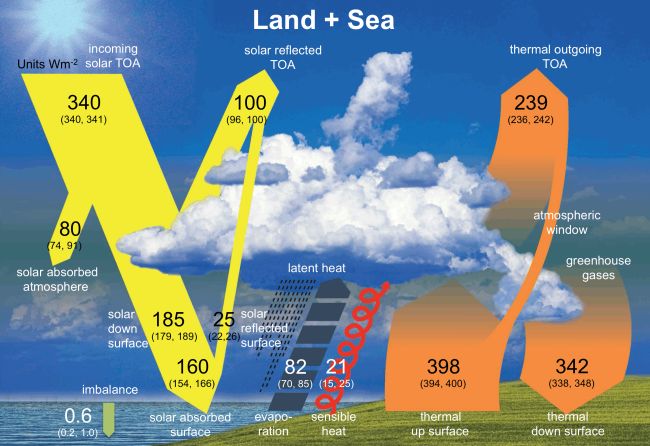
Figure 2. Schematization of Solar / Troposphere / UOS and land. The thickness of the red and yellow bands is representative of the flows indicated, expressed in W/m2. Source: Wild et al[34].

 

Let us now specify the hypotheses, the notations used and the relations which will intervene:

We assume that from month to month the mass of water present in the UOS remains constant, with precipitation compensating for evaporation.

 

We will denote by Cn the quantity of heat acquired or lost during month n by the UOS and by θn its average temperature in month n by the UOS and by θn its mean temperature in month n.

 

θn and therefore Cn mainly undergo five influences:

(1) That of the sun, by supposedly constant radiation but tempered by the cloudiness which generates the atmospheric albedo effect.

 

(2) That of the sensible heat of the atmosphere of temperature tn by contact.

 

(3) By the cooling caused by evaporation on the surface of the UOS.

 

(4) By long-wave radiative heat flux to the atmosphere.

 

(5) Through heat exchanges with the lower ocean layer, the thermal insulation between the UOS and its lower zone not being absolute.

 

Similarly, the quantity of heat acquired or lost during month n by the Troposphere will be denoted Tn and tn its average temperature during month n.

 

tn and therefore Tn are subject to four influences:

(1) By contact, that of the sensible heat of the surface of the UOS.

 

(2) By radiation tempered by cloudiness and the atmospheric albedo effect, that of the sun.

 

(3) By the warming caused by the latent heat transported by the water of the UOS which evaporates and which is released into the atmosphere when it condenses to eventually form clouds and bring precipitation.

 

(4) By the greenhouse effect caused in particular by water vapor and other greenhouse gases which trap part of the infrared radiation coming from the surface of the UOS.

 

During month n, the energy balance of the UOS corresponds to the difference between the energy received and the energy lost during this period. It translates to this equation:

 

 

And similarly, that of the Troposphere corresponds to this relationship:

 

 

With:

(1) Cn being the heat accumulated by the UOS during month n.

 

(2) Tn representing the heat accumulated by the Troposphere during month n, Rg noting the energy coming from the monthly global radiation of solar origin. It is assumed to be constant. Starting from the power value given by Poitou[35], of 340W/m², we obtain Rg=340×3600×24×30=881,280,000J/m², which we round up to 9×108J/m².

 

(3) an being the average atmospheric albedo in percentage of the planet during month n. So the expression (100-an) Rg corresponds to the part of the solar energy not reflected outside the Troposphere following the atmospheric albedo effect.

 

(4) bn denoting the percentage of Rg radiation which is not reflected outside the Troposphere by atmospheric albedo effect, but absorbed by it before arriving at the surface of the UOS. So the expression bn Rg corresponds to the part solar energy trapped by the Troposphere before reaching the surface of the UOS.

 

(5) Ren= Rsn - Ran representing the effective thermal infrared radiation emitted during month n. It is equal to the difference between the thermal infrared radiation Rsn emitted by the ocean surface and that Ran of the atmosphere.

 

(6) Kn being the sensible heat exchanged with the air during month n.

 

(7) K'n representing the sensible heat exchanged with the lower layer during month n.

 

(8) Vn denoting the amount of water evaporated during month n.

 

(9) l is the latent heat of vaporization of water. We will take its value for a temperature close to 15°C at atmospheric pressure, i.e., approximately 2,470kJ/kg.K.

 

(10) σn corresponding to the percentage of the energy En=lVn necessary for this evaporation and which was not drawn from the ambient air but from the UOS.

 

Below, some additional details concerning what comes into play in relations (1) and (2):

(1) Given the significant thermal inertia of the oceans and the thermal phase shift of around three months that it causes (Le Calvé[20]), we will start from the following expression of the heat accumulated in the UOS: Cn=Cdyn (θn+3-θn+2) where Cdyn designates what we call the "dynamic heat capacity" of the UOS and θn its average temperature during month n. The classic heat capacity of still water at the temperatures involved is approximately C=4.18kJ/kg.K and since, according to Le Calvé[20], the average height of the UOS is about 100m, the heat capacity per m2 of surface of this UOS is therefore approximately 4×108J/K. But the water in question here is in constant movement movements caused by the winds, the tides and the currents, and thus this constant forced convection of the heat which arrives by the sun acts as if the water of the UOS had a much greater heat capacity than in the case of still water. We obtained an estimate of this constant by "calibrating" the model with the observations (see line 3 of Table 7). Also note that this concept of dynamic heat capacity makes it possible to integrate into our model the influences of phenomena such as currents, winds or tides, even if in a very rudimentary way. From observations made on the temperatures of mountain straims[36], we justify and specify this concept in Appendix 1.

 

(2) To assess the "observed" temperature of the UOS denoted Θn from the An anomalies of ocean heat studied above, we will use the following relationship: Θn+1=Θn+c(An+1-An). To estimate the previous constant c, we first use an estimate of the decadal increase in ocean heat obtained from the data previously studied (see paragraph 2.3). That is about 3.3u. per decade (where 1u.=1022J). Then, for the same period 1955-2022, we know from National Oceanic and Atmospheric Administration that for the upper ocean layer between 0 and -75m (roughly what we call the UOS), the average temperature increase is about 0.11°C per decade. We will therefore take c=0.11/3.3=1/30.

 

(3) We will denote by Tan the temperature of the atmosphere obtained directly using their anomalies Bn studied above by this relationship: Tan+1 = Tan+ (Bn+1-Bn).

 

(4) The thermal inertia of the Troposphere is weaker than that of the UOS, but nevertheless real: in France, for example, the hottest month of summer is not the one with the longest days and therefore potentially the sunniest (June), but late July / early August, so with a thermal phase shift of a good month. Similarly, the coldest month is not the one with the shortest days (December), but rather the period mid-January-early February. We will therefore start from the following expression for the heat accumulated in the Troposphere: Tn = C’dyn (tn+1-tn) where C’dyn is the "dynamic heat capacity" of the Troposphere and tn its average temperature during the month not. The classic heat capacity C' of still air is about 1kJ/kg.K and with an average height of the Troposphere around 10,000m, the heat capacity per m2 of cross-sectional area of a column of this UOS is therefore about 108J/K (density of the air at the temperatures in question: about 1kg per cubic meter). Much more than the water in the UOS, this air is subject to constant movement, in particular due to atmospheric winds and upward or downward convection caused in particular by the temperature differences that are created in the Troposphere. We again obtained an estimate of this constant by "calibrating" the model with the observations (line 4 of Table 7).

 

(5) According to Poitou[35], the share of energy of solar origin trapped by the atmosphere before reaching the surface of the planet represents approximately one third of all of this solar energy not returned to the atmosphere space by the albedo effect. What we translated by the following relation: bnRg = (100 - an)Rg.

 

(6) According to the Stefan-Boltzmann law, the infrared radiation Rsn emitted by the ocean surface evolves according to the fourth power of the temperature expressed in Kelvin degrees. This leads to a relation of the type Rsn=α×tn4, with which we obtain the following approximation: where ε = tn+1 - tn. We will use this approximation in our model.

 

(7) Loeb et al.[37] observe that the radiation Ran retained by the greenhouse effect increases following in particular and above all the increase in evaporation caused by global warming. We will therefore take the following relation:

 

(8) However, the study of data from Rossow[38] highlights a decrease of about 1% per decade in low cloud cover for the period 1984-2009. At the same time, the temperature of the atmosphere was increasing by around 0.1°C per decade. This shows that the increase in radiation Ran retained by the greenhouse effect is not fully compensated by the increase in Rsn caused by warming; and therefore the effective infrared radiation Ren=Rsn-Ran decreases.

 

Moreover, as the significant atmospheric albedo effect caused by low cloudiness decreases at the same time as the latter is reduced, the net solar radiation Rg (100-an) towards the surface of the oceans increases. This causes an energy imbalance of the Earth between these two types of radiation, weak (of the order of 0.3% according to Loeb et al.[37]), but real. And this imbalance largely explains the two phenomena described in paragraph 2.3: On the one hand the warming of the oceans, and particularly that of the UOS, of approximately 3×1022J per decade for the period 1984-2009. On the other hand, the warming of the atmosphere, at a rate of approximately 0.1°C per decade for the same period.

 

(9) According to Mendoza et al.[39] where thermodynamic arguments are used, there is an inverse proportionality between cloud cover and the temperature of the Troposphere. What we translate by the following relation: .

 

(10) If θn≥tn, the water from the UOS loses sensible heat to the air layer above it and Kn=kT(θn-tn), where k is proportional to air effusivity and T=3600×24×30T=2,592,000s. is the duration of a month expressed in seconds. If θn<tn, the UOS gains sensible heat from the air layer above it and Kn=k’T(θn-tn), where k' is proportional to the thermal effusivity of water. The effusivity of air being 6JK-1 m-2 s-1/2 and that of water being 1590JK-1 m-2 s-1/2, we will take k=6 and k'=1590. For the chosen proportionality constant (i.e. 1), we obtained it by adjusting this constant as well as possible to the known average of sensible heat (20W/m² according to Poitou[35], i.e. 20×T= 51840000J per month and per m2).

 

(11) The water below the UOS has a temperature constantly lower than θn so the sensible heat exchange always goes in the direction of the UOS to the lower layers. But due to the strong oceanic stratification, this exchange is weak and moreover tends to decrease further because this stratification phenomenon is further accentuated with climate change (Li et al.[22]). Moreover, this heat exchange by conduction is accentuated when the temperature of the UOS increase. To evaluate it, we will therefore use the relation K’n where K’1 is the heat loss of the UOS towards the lower layer in the first month of our modeling and sn the coefficient which takes into account the accentuation of the current stratification of around 1% per decade since 1971 (Li et al.[22]). We will therefore take sn=(1.011/120)n. As for the estimate of K'1, we obtained it by "calibrating" the model with the observed data (see line 8 of Table 7).

 

(12) The rate of vaporization of a water surface, modeled for example by Stefan's law of evaporation or by Penman's formula (Belarbi and Saighi[40]), increases with the temperature of the water, and decreases with the humidity of the surrounding air. A rise in air temperature tends to lower the relative humidity. The amount of water Vn that evaporates on the surface of the UOS is therefore an increasing function of θn and tn. Even if these variations are not linear, taking into account the very small amplitudes of the intervals over which these two temperatures move, a modeling of Vn by a function of the form β θn tn seemed to us to sufficiently account for reality with respect to the objectives to be achieved by our model. We will also use the relation .

 

(13) To determine the share σn of the energy required for vaporization taken from the UOS compared to all of this energy, we started from the following observations: The air-sea temperature at the surface is often slightly to the advantage of the water of the UOS compared to the air located immediately above[20]. So the very important energy necessary for the evaporation of En is drawn much more from the UOS than on the outside. This is even the most important cause of its cooling[20]. Moreover, the drop in temperature of a body of immobile water that is not subject to external bad weather provides a good order of magnitude of the quantity that has evaporated there (Albertson[41]). However, a significant part of this energy is also drawn from the heat of the ambient air, especially for periods and places subject to summer heat where the temperature of the UOS is often much lower than that of the ambient air: the atmosphere close to the surface of the water then constitutes a significant source of calories capable of generating this evaporation. On the other hand, in places subject to the rigors of winter, it is rather the temperature of the UOS which is higher than the one of the ambient air, and in this case the energy necessary for the vaporization is all the more taken in the UOS. This is what, in our opinion, largely explains the large variations that it is in the evaporative heat flux leaving the UOS: according to Le Calvé[20], its annual average is -90W/m² while varying between -160 and -50W/m2. We will also use in our model the following expression of the percentage of vaporization energy taken directly from the UOS: σn=-0.1tn+0.8+0.1θn. For example, if the temperature θn of the UOS exceeds the temperature tn of the atmosphere by 1°C, this expression of σn gives a result of 90% for the vaporization energy drawn from the UOS, and therefore 10% for that drawn from the ambient air. If on the contrary θn is lower by 1°C than the temperature tn we obtain 70% for the UOS and 30% for ambient air. If finally θn=tn we obtain 80% for the UOS and 20% for ambient air. There is of course a large part of arbitrariness in this empirical expression of σn, but we believe that we have taken into account the above as well as possible, in particular the fact that in any month of the year, there is always a part not insignificant part of the planet which is subject to the rigors of winter, and another subject to strong summer heat.

 

The following table summarizes the relationships justified and explained above and which will be used for our modelling:

 

Table 7. Summary of the Relationships Founding the Model and Complementary Relationships

 

We present in Figure 3 an example of simulation obtained with the previous relations by a discrete modeling implemented on a simple spreadsheet (Excel). The period for the observations covers from January 1955 to December 2022, i.e. 804 months, that for the simulations also starts in January 1955 and ends in December 2095, i.e. 1680 months.

 

(1) The red curve gives the variations in temperature Tan observed in the atmosphere.

 

(2) The purple curve those of tn obtained by the model.

 

(3) The blue curve gives the temperature variations Θn observed in the UOS.

 

(4) The green curve those of θn obtained by the model.

 

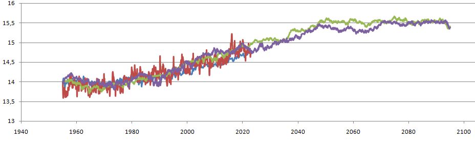
Figure 3. Simulations of tn and θn over the period 1955-2095 compared to the temperatures observed Tan and Θn during the period 1955-2022. Red curve: observed atmospheric temperature Tan. Purple curve: simulated atmospheric temperatue tn. Blue curve: observed upper ocean layer temperature Θn. Green curve: simulated upper ocean layer temperature θn.

 

The Table 8 specifies the average lengths of the chains at play and the correlations between the different types of data over their common periods.

 

Table 8. Average Lengths of the Climb Chains for the Observed Data (Period 1955-2022) and for the Data Resulting from the Simulation (Period 1955-2095)

Notes: Correlation coefficients between different types of data over their common periods.

 

As clearly confirmed by the correlation coefficients, the simulation is well aligned with the real variations over their common period 1955-2022. Moreover, there is a good correlation between the two types of data simulated over the period 1955-2095, as good as between the two types of data observed over the period 1955-2022. As for the average lengths of the climbing chains, they are compatible with the observed reality.

 

Remarks:

(1) Natural variability was taken into account by introducing random coefficients into the calculations of θn and tn by our model. The ranges of possible variations of these coefficients take account of the variations actually observed.

 

(2) These coefficients simulate random variations subject to a uniform law. So if there is no correction in the model, the chains of ups and downs associated respectively with θn and tn would behave as if they were managed by a binomial law, which we have seen is not realistic. To correct this, we added a random weighting to the model which very slightly increases the probability of reversal of a deviation of θn and tn and very slightly decreases those that they do not reverse. The average lengths of the ascent and descent chains take values compatible with those of the observations.

 

(3) In this regard, by studying the monthly fluctuations involved of the temperatures θn and tn resulting in these chain lengths consistent with the observed results, we have found that they are of the order of a thousandth of a °C. So in our opinion the phenomenon of forced alternation that we detected by the study of the distribution of the climbing chains had practically no possibility of being detected directly from simulations from global climate models, as elaborate and precise be they.

 

(4) We present in Appendix 2 two other simulations accompanied by the table of characteristic values to be able to compare with the observations. We still note the good rendering of these simulations compared to the observations. In addition, this illustrates the great ease and speed of obtaining correct simulations thanks to this model.

 

(5) For any request that he deems justified, the author will provide a copy of the model file free of charge by e-mail.

 

3.4 Origins of the Acceleration of Climatic Nervousness Observed from 1970

Let us first recall what was reported on this question in Zeltz[6]: The forced alternation of rises and falls of deviations of monthly anomalies of the global average atmospheric temperature accelerates considerably from 1970 since for the period 1880-1970, the chains of rises have an average length between 1.6 and 1.7, including for the period of strong warming which goes from 1911 to 1945, whereas from 1970 this average drops to 1.47.

 

What is different and makes that, even with such a rapid warming, the period 1911-1945 alternates less rapidly than the current period since 1970?

 

As we will explain next, we believe that this is the increase in ocean stratification since the 1960s that is mainly responsible for this phenomenon. According to Li et al.[22], this has increased by more than 5% in recent decades (1960-2018), or about 0.90% per decade. Most of the increase (more than 70%) having occurred in the upper 200m of the ocean, meaning precisely what we have called the UOS. Still according to Li et al.[22], it is above all changes in temperature that are responsible for this phenomenon, even if changes in salinity locally can sometimes play an important role.

 

When the UOS heats up, due to the fact that mixing vertical in particular has down significantly due to the increase in stratification[22], physical exchanges and therefore also thermo-convective exchanges between the thermocline and the UOS are attenuating. The evacuation of excess calories from the UOS to the atmosphere can therefore only increase in the form of latent heat by additional evaporation. Then, the additional cooling that it causes in the UOS slows all the more vigorously down during the next evaporation phase. However, we have seen previously that it is the main player in the mechanism at the origin of the forced alternation of atmospheric temperature. And so, since the increase in stratification accentuates both the power and therefore the speed of increase and decrease of this evaporation, it follows that the alternating rise / fall of the average of the anomalies of the global atmospheric temperature accelerates at the same time as this stratification rises.

 

4 CONCLUSION

Starting from the observation of "forced alternation" of average monthly atmospheric temperatures worldwide which was made in Zeltz[6], we show that the phenomenon that we call "natural climatic nervousness" is the result of an interaction between the first oceanic layer and the troposphere, an interaction whose engine is two-step: the cooling-warming of the UOS related to evaporation.

 

Then, the discordance of the periods of the forced alternations observed between the atmospheric temperature (of the order of a month) and that of the heat stored in the first oceanic layer (of the order of a quarter) is explained on the one hand because of the large thermal inertia of ocean water, on the other hand due to the imbalance of monthly increases and decreases in atmospheric temperature which feed the quarterly thermal balance of the UOS: with our notations, DAD quarters alternate with ADA quarters.

 

Finally, the acceleration in the speed of forced alternation from the 1970s is explained by taking into account the increase in ocean stratification observed since 1960.

 

This article first shows the great interest of the approach of a probabilistic study of the time series involved: it makes it possible to identify phenomena which are undoubtedly very difficult to detect by the methods usually used in climatology. In our case, "signals" as simple as the greater or lesser average lengths of the climbing chains allowed us to test and ultimately reveal with great precision interactions that would not have been understood otherwise, or much more superficially.

 

As for the model described in this article, based on the ocean / atmosphere energy balances and integrating our probabilistic findings, it proved capable of making fairly good simulations of global atmospheric and ocean temperatures, largely consistent with observations. This model therefore already seems interesting to us in its current state, but, equipped with a few additional refinements and improvements, it would undoubtedly constitute a tool that is both very simple and quick to use, but also reliable in the results it would give. This would allow non-specialists in climatology equipped with a minimum of scientific culture to really grasp the reality of climate change, much better than by the almost blind confidence that they must for the moment give to the results appearing in the reports of the major climatological institutes. These results come in fact for the most part from global climate models that are inaccessible to most non-specialists:

(1) Already by the masses of properly climatological knowledge that they require for their full understanding. This even if a major effort to popularize this knowledge has been provided for a few years (see for example Gettelman and Rood[21]).

 

(2) Then, by the lack of transparency in the modeling exercise and the data used, which also limits the understanding and interpretation of the results (observation made by Hache et al.[42] for the integrated assessment models energy-climate-economy, but which remains true for the vast majority of global climate models, if not all).

 

(3) Finally, by the need to have a very high-powered computer at your disposal and a lot of time to obtain a simulation yourself.

 

While continuing the probabilistic study of reliable climate data series by the techniques used here, this will encourage us to continue working with the aim of improving this model, while scrupulously ensuring that it remains accessible to non-users specialists for its understanding and use.

 

Acknowledgements

I sincerely acknowledge Jérôme Pousin and Jean Poitou for their proofreading of the manuscript and their valuable advice.

 

Conflicts of Interest

The author declared that there is no conflict of interest regarding the publication of this article. No potential conflict of interest has been reported by the author.

 

Author Contribution

The author participated in the drafting and writing of the manuscript. The author contributed to the manuscript and approved the final version.

 

Abbreviation List

ADA, Ascent, Descent, Ascent

DAD, Descent, Ascent, Descent

UOS, Upper oceanic stratum

 

References

[1] Webster PJ. The role of hydrological processes in ocean‐atmosphere interactions. Rev Geophys, 1994; 32: 427-476.[DOI]

[2] Bony S, Dufresne JL. Marine boundary layer clouds at the heart of tropical cloud feedback uncertainties in climate models. Geo Res Lett, 2005; 32: L20806.[DOI]

[3] Peng Q, Xie SP, Wang D et al. Coupled ocean-atmosphere dynamics of the 2017 extreme coastal El Niño. Nat Commun, 2019; 10: 298.[DOI]

[4] Chelton DB, Xie SP. Coupled ocean-atmosphere interaction at oceanic mesoscales. Oceanogr, 2010; 23: 52-69.[DOI]

[5] Delmas JF. Stochastic Processes and Applications. Accessed 2023. Available at:[Web]

[6] Zeltz É. Analyse et interprétation climatologique de l'évolution des températures moyennes mondiales depuis 1880. Physio-Géo. Phys Geog Environ, 2021; 16: 49-70.[DOI]

[7] Lorenz EN. Deterministic nonperiodic flow. J Atmos Sci, 1963; 20: 130-141.[DOI]

[8] Le Treut H, Jancovici JM. L’effet de serre: Allons-nous changer le climat? Flammarion: Paris, France, 2009.[DOI]

[9] Shukla J. Dynamical Predictability of Monthly Means. J Atmos Sci, 1981; 38: 2547-2572.[DOI]

[10] Pailleux J. Quelle est la différence entre météorologie et climatologie? Accessed 2023. Available at:[Web]

[11] Buizza R, Leutbecher M. The forecast skill horizon. Q J Roy Meteor Soc, 2015; 141: 3366-3382.[DOI]

[12] Stock CA, Pegion K, Vecchi GA et al. Seasonal sea surface temperature anomaly prediction for coastal ecosystems. Prog Oceanogr, 2015; 137: 219-236.[DOI]

[13] Shi H, Jin FF, Wills RCJ et al. Global decline in ocean memory over the 21st century. Sci Adv, 2022; 8: eabm3468.[DOI]

[14] Hamilton JD.Time Series Analysis. Princeton University Press: Princeton, USA, 1994.

[15] USA. National weather Service. Climate Prediction Center. Cold & Warm Episodes by Season. Accessed 2023. Available at:[Web]

[16] Kim WM, Cai W. Second peak in the far eastern Pacific sea surface temperature anomaly following strong El Niño events. Geo Res Lett, 2013; 40: 4751-4755.[DOI]

[17] Self S, Zhao JX, Holasek RE et al. The Atmospheric Impact of the 1991 Mount Pinatubo Eruption. Accessed 2023. Available at:[Web]

[18] Cherian R, Quaas J, Salzmann M et al. Pollution trends over Europe constrain global aerosol forcing as simulated by climate models. Geo Res Lett, 2014; 41: 2176-2181.[DOI]

[19] Nabat P, Somot S, Mallet M et al. Contribution of anthropogenic sulfate aerosols to the changing Euro‐Mediterranean climate since 1980. Geo Res Lett, 2014; 41: 5605-5611.[DOI]

[20] Le Calvé O. Propriétés Physiques du Milieu Marin. Un cours d'introduction à l'océanographie physique. Accessed 2023. Available at:[Web]

[21] Gettelman A, Rood RB. Demystifying climate models: A users guide to earth system models. Springer Nature, 2016.[DOI]

[22] Li G, Cheng L, Zhu J et al. Increasing ocean stratification over the past half-century. Nat Clim Change, 2020; 10: 1116-1123.[DOI]

[23] El Khatri S. Manuel du cours de Climatologie. Direction de la Météorologie Nationale Centre National de Recherches Météorologiques. Casablanca. Accessed 2023. Available at:[Web]

[24] Giorgi F. Climate change hot‐spots. Geo Res Lett, 2006; 33: L08707.[DOI]

[25] Wyant MC, Bretherton CS, Blossey PN. Subtropical low cloud response to a warmer climate in a superparameterized climate model. Part I: Regime sorting and physical mechanisms. J Adv Model Earth Sy, 2009; 1.[DOI]

[26] Meehl GA, Arblaster JM, Tebaldi C. Understanding future patterns of increased precipitation intensity in climate model simulations. Geo Res Lett, 2005; 32: L18719.[DOI]

[27] Le Barbé L, Lebel T. Rainfall climatology of the HAPEX-Sahel region during the years 1950-1990. J Hydrol, 1997; 188: 43-73.[DOI]

[28] Blandford TR, Humes KS, Harshburger BJ et al. Seasonal and synoptic variations in near-surface air temperature lapse rates in a mountainous basin. J Appl Meteorol Clim, 2008; 47: 249-261.[DOI]

[29] Bonnardot V, Carey VA, Madelin M et al. Spatial variability of night temperatures at a fine scale over the Stellenbosch wine district, South Africa. OENO One, 2012; 46: 1-13.[DOI]

[30] Vial J, Albright AL, Vogel R et al. Cloud transition across the daily cycle illuminates model responses of trade cumuli to warming. P Natl Acad Sci USA, 2023; 120: e2209805120.[DOI]

[31] Lubes H, Masson JM, Servat JE et al. Caractérisation de fluctuations dans une série chronologique par applications de tests statistiques Etude Bibliographique. Accessed 2023. Available at:[Web]

[32] Levitus S, Antonov J, Boyer T et al. World ocean heat content and thermosteric sea level change (0-2000m), 1955-2010. Geo Res Lett, 2012; 39: L10603.[DOI]

[33] Levitus S, Antonov J, Boyer T. Warming of the world ocean, 1955-2003. Geo Res Lett, 2005; 32: L02604.[DOI]

[34] Wild M, Ohmura A, Schär C et al. The Global Energy Balance Archive (GEBA) version 2017: A database for worldwide measured surface energy fluxes. Earth Syst Sci Data, 2017; 9: 601-613.[DOI]

[35] Poitou J. Composition atmosphérique et bilan radiatif. Reflets de la Physique, 2013; 33: 28-33.[DOI]

[36] Bocquet G. Les températures des eaux et leur évolution dans le bassin d'alimentation de la haute Romanche (Mesures et essai d'interprétation). Accessed 2023. Available at:[Web]

[37] Loeb NG, Johnson GC, Thorsen TJ et al. Satellite and ocean data reveal marked increase in Earth’ s heating rate. Geo Res Lett, 2021; 48: e2021GL093047.[DOI]

[38] Rossow WB, Walker AW, Beuschel DE et al. International satellite cloud climatology project (ISCCP) documentation of new cloud datasets. Accessed 2023. Available at:[Web]http://isccp.giss.nasa.gov/docs/documents.html

[39] Mendoza V, Pazos M, Garduño R et al. Thermodynamics of climate change between cloud cover, atmospheric temperature and humidity. Sci Rep, 2021; 11: 21244.[DOI]

[40] Belarbi N, Saïghi M. Etude comparative des méthodes d’évaluation du taux d’évaporation à partir d’une surface d’eau libre. Application aux régions arides et semi arides en Algérie. Accessed 2023. Available at:[Web]

[41] Albertson ML. La mécanique de l’ évaporation. Accessed 2023. Available at:[Web]

[42] Hache E, Simoën M, Seck GS et al. Comprendre les enjeux de la modélisation du lien complexe entre energie, climat et économie. Accessed 2023. Available at:[Web]

&nbsp;

Copyright © 2023 The Author(s). This open-access article is licensed under a Creative Commons Attribution 4.0 International License (https://creativecommons.org/licenses/by/4.0), which permits unrestricted use, sharing, adaptation, distribution, and reproduction in any medium, provided the original work is properly cited.