Using Household Electricity Metrics in Identifying Trends in Residential Appliances Usage in Selected Ghanaian Homes

 

Timothy King Avordeh1*, Christopher Quaidoo2, Samuel Arthur2

 

1Research and Consultancy Centre, University of Professional Studies, Accra, Ghana

2Department of Banking and Finance, University of Professional Studies, Accra, Ghana

 

*Correspondence to: Timothy King Avordeh, PhD, Research Fellow, Research and Consultancy Centre, University of Professional Studies, New Rd, Accra 00233, Ghana; E-mail: timothy.avordeh@upsamail.edu.gh

 

DOI: 10.53964/jmge.2022006

 

Abstract

Objective: The paper aims to clarify the association between consumption trends for four appliance types and power consumption in residential facilities in selected buildings in Ghana. It proposes modelling the consumers’ consumption demand process and outlining why and how appliance use in residential homes is important throughout the energy supply system and consumer expectations for improved energy quality process. Integrating the various aspects of saving electricity, this analysis provides a comprehensive overview of the factors that contribute to successful energy-saving behaviour the study seeks to recognize the need for a comprehensive approach to achieving energy reduction targets, incorporating household dynamics and behaviors to identify the root causes of energy-saving behavior than is normally found in the home appliance consumption trends in literature.

 

Methods: The residential household survey dataset fulfilled the research criteria by analyzing data from 100 households and about 1007 individual household electrical appliances. The tracked data includes accurate data of different electrical appliances used in the selected homes, and consumption data over a duration of one year. Several computer programming languages and software methods have been used to build the stochastic demand model for the trend analysis. Anaconda software especially the RStudio and MATLAB are used to define indicators of customer behaviour, analyze the dataset for the chosen home appliances and examine the impact of appliance use on the household dataset. The model (household types, appliance ownership, and electricity demand) has been introduced in the MATLAB language. The agent-based model is introduced to capture realistic individual-level behavior patterns and coordinated reactive changes in human behavior in order to better predict the reduction dynamics of consumption of electricity in residential homes.

 

Results: The paper provides empirical evidence on how behavioral changes through the study of appliances help reduce household electricity. The results showed that the consumption behavior of devices for individuals is correlated with each other. The refrigerators had the most switch-on events in a day, and the refrigerator had the most power-ups in a day. This happens because the compressor works continuously throughout the day. Television has the longest usage time per device, with the average user watching TV 230min per week. The refrigerator (178.6min) and laptop (14.6h, 175.8min) follow next. Grill had the shortest duration per use, averaging 2.4min across the 30 video channels in the given dataset. The results also show that there is no statistically significant difference between household types, number of residents or types of day. With the reduction in household electricity consumption, this is clearly a regenerative path with new economic thinking in areas such as technological advancement and societal awareness.

 

Conclusion: Due to the research approach, the research results may lack generalizability. Therefore, researchers are encouraged to further test the proposed proposals. Practical Implications: The paper contains implications for the development of a trend consumption model. Government agencies must carefully define their consumption adjustment supports and incentive programs to influence consumption practices and demand management at the residential level. Here, energy policy and investments need to be more strategic. The most critical problem is to identify the appropriate adaptation strategies that benefit the most vulnerable sectors such as housing. What is the Original/Value of Paper: This paper fills an identified need to explore how consumer consumption behavior can be modeled.

 

Keywords: residential electricity, household consumption, energy sector, smart meters monitoring, consumer behavior, metrics

 

1 INTRODUCTION

In modern society today, access to energy, more importantly, electricity, has in recent years received ever greater attention globally by governments and utility players. Electricity demand to a large extent mirrors all three aspects of the sustainable development of every country; political, social, and environmental considerations. This growing global concern is captured more succinctly in the sustainable development goal (SDG): which requires governments to make available energy for all their citizens at all times through modern, affordable, reliable, and sustainable supply. Electricity is the most widely used modern-day energy source in Ghana, accounting for around 48% of the energy consumed in the industrial and commercial sectors and approximately 52% in residential consumption[1]. The government’s electricity and climate change objectives are to make available to consumers secure electricity on the way to a sustainable supply for demand into the future and drive determined action on climate change at home. To make sure this agenda becomes a reality, the government deems it most critical that we address both security and supply challenges while taking advantage of maximizing the benefits and minimizing costs for consumers at large. It is only in the electricity sector wherein the government’s energy policy are these challenges more evident.

 

In the electricity sector, ensuring unending security of supply of generation and maintain affordability is particularly the challenging situation in Ghana today. Moreover, electricity demand is set to expand over the coming decades as major sectors such as domestic and manufacturing are electrified. Indeed, to meet these challenging situations an estimated £110 billion of investment in electricity generation and supply is needed in this decade alone[2]. Their study indicates that around £75 billion in new energy production capacity may be required, whereas Ofgem’s “project discovery” estimates that approximately £35 billion in extra investment is required for electricity transmission and distribution[3]. Figure 1 summarizes the government’s goals for the electricity sector.

 

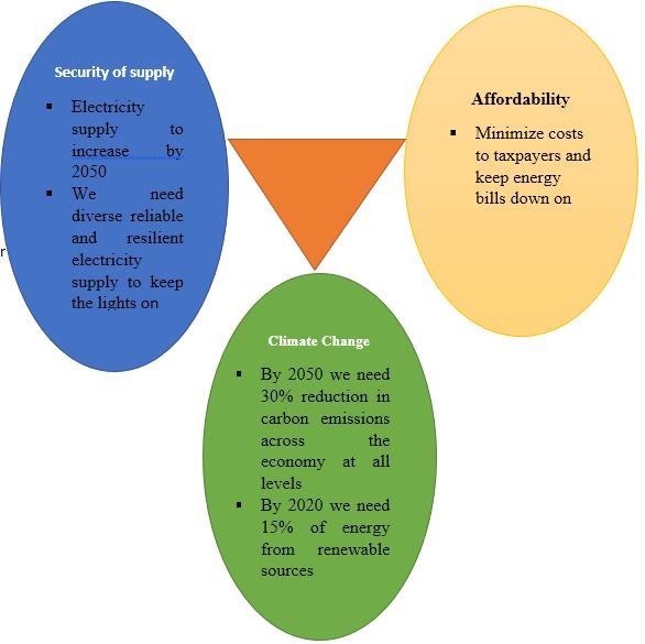
Figure 1. The government’s objectives for the electricity security system.

 

According to National Energy Statistics from Energy Commission of Ghana[4], given the increase in generation capacity experienced following the first electricity crisis in 1982 and 1984, there was a serious drought, as the overall Akosombo Dam’s inflow was less than expected. As a result of this crisis, thermal power plants (TPP) were integrated into the generation mix of Ghana. The first of these thermal plants at Takoradi Thermal Plant, operated by the Volta River Authority (VRA), was a 550MW facility (Tapco and Tico). The installed capacity of TPP in Ghana increased to 3,456MW as of the end of 2019, which is 2,906MW from the present peak. The projected total thermal energy generation for 2019 is 11,460.11GWh from VRA plants and (independent power producers) IPPs[5]. The locally accepted word “dumsor” has become the adopted word for the situation in Ghana since the energy crisis became a household phenomenon. The country’s entire economic situation was affected, so in December 2013 Bui hydroelectric power station with 400MW was commissioned to supply electricity to meet the country’s peak load, which has been on an ever-increasing trajectory.

 

Ghana’s power market, which was formerly regulated by the public sector, is said to have shifted from hydro to thermal. Main concerns in the sector include demand exceeding production, inadequate transmission and delivery, the government’s control of IPPs, and tariffs that do not cover costs. Ghana, with the help of international donors, decided to reinforce the electricity sector faced with. The government has identified two main goals for addressing the sector’s current issues and enabling it to achieve long-term, sustainable economic growth: First, double installed generation capacity and second, expand universal access to electricity by 2020. The result is shown in Adom’s research[6]. The government over the years have attracted more private sector participation in the sector. IPPs have therefore taken over the electricity generation market. Efficiency technologies[7], modification of consumer behaviors, which refers to accepting actions to reduce electricity consumption, to make it possible for consumers to vary their patterns of electricity consumption and adopt new habits. This allows consumers in eliminating wasteful consumption of electricity such as turning off a light when leaving a room. This group of measures does not require consumers to change their domestic electricity demand patterns, like the application of various types of insulation or using energy-saving lighting. According to studies by Ahmed et al.[8], “efficient” behavior is generally favored above “curtailment” behavior because of the higher potential for electricity savings. Because technical advances can achieve the maximum potential for households’ power consumption reduction by 2020, which is estimated at 47%[9], which estimates show will rise to 35% by 2020, as US consumers use less electricity to save money[10].

 

The aggregated demand for electricity from home appliances is a major part of the household consumption according to Strbac et al[11]. Home appliances are also one of the main tools for demand-side elasticity. The combined impact of market changes may be accomplished by preparing equipment for another time of day. The emphasis should therefore be on the level of household equipment, the management and optimization of their activities[12,13]. Solid knowledge of home appliances and the user behavior which determines household energy demand, are required to measure the capacity of demand responses. This is also critical because the ties are useful for developing a practical energy demand model for household appliances. Demand for energy in homes and future demand response depends on three major factors: Household electrical appliances ownership, consumer behavior and the electricity demand characteristics of household appliances, and the suitability of appliances for a response to demand.

 

The objective of this study is to determine consumption trends for four appliance types to determine the existing use of power consumption in residential facilities in selected buildings in Ghana. The research paper tries to answer the main question what are the consumption trends of appliances on consumers’ demand in residential facilities. Ghana’s energy demand has been impacted by inefficiencies in the energy supply and consumer expectations for improved energy quality, and these two factors have harmed Ghana’s energy supply and reliability. Electrical demand is an econometric trend that necessitates improved energy efficiency, together with supportive policies to help reduce network inconvenience and encourage lower electricity prices. However, this assumption is essential and concrete, and, as a result, lacks proper policy solutions and associated boundaries. Behavioral techniques are of course part of the effort to introduce more energy-efficient solutions as well as new technology within the energy sector. In Ghana, electricity demand is highest in the residential sector where a lot of appliances are used for their daily comfort.

 

Reduction in electricity, asset preservation, and environmental preservation will be critical, necessitating major behavioral changes in households, businesses, and products[14]. The determinants of observed and reported household behavior are investigated in this study, which adds to the environmental literature on energy demand and saving behavior. The body of knowledge about the key factors influencing power usage and household energy-saving habits is growing[15-17]. This latest study’s results support the claim that behavioral approaches to energy policy can be beneficial. Because of its immense energy-saving capacity, the residential sector was a primary priority for energy conservation policies. Many reports show that the residential sector has the highest ability to reduce electricity demand and greenhouse gas pollution in a long-term, beneficial, and cost-effective way. According to the International Energy Agency, non-technical obstacles prevent approximately 80% of the economic energy-saving potential in buildings from being realized. Furthermore, despite the focus on energy-saving actions as a tool for energy conservation, our understanding of their drivers and their effect on household energy demand remains limited. The findings of such studies, on the other hand, are mixed. Our research paper sheds new light on the factors affecting household energy conservation.

 

This highlights the significance of observational research in understanding household energy-saving behaviors and the relationship between socioeconomic needs and residential characteristics. The residential sector accounts for about 30% of overall energy consumption and 20% of CO2 emissions[18]. Enhancing the efficiency of existing household appliances is also one of the most cost-effective means of lowering greenhouse gas and pollutant emissions. As a result, learning more about the factors that drive a reduction in domestic energy consumption would favor both the economy and the climate. Following the hosting of COP21 and the global adoption of the Paris Climate Convention, the French government has introduced a new strategy known as the Electricity Transformation with Green Growth Bill[19], which sets an optimistic target for the domestic economy to dramatically decrease reduction while decreasing cost. As stated earlier the primary aim of the objective of this research paper is to accelerate the basic rehabilitation of the current housing standard. To promote this energy transition and achieve significantly lower energy demand in the housing sector, the French Ministry for Ecological and Solidary Transformation has implemented a range of financial benefits and regulatory instruments: I make it simple to obtain zero-interest loans[20]. Households and buildings, access to energy supply, environment, household appliances, and efficiencies, energy sources, and energy policy are all factors that affect how electricity is used in homes. Behavioral and attitude-based energy savings have been described as significant gaps in our understanding of the residential energy market. They do have tremendous potential for lowering domestic energy use. As a consequence, behaviors, and attitudes are regarded as critical factors affecting the use and spread of energy-saving technologies, as well as the long-term sustainability of energy systems[21].

 

This study recognizes the need for a comprehensive approach to achieving energy reduction targets, incorporating household dynamics and behaviors to identify the root causes of energy-saving behavior. By integrating the various aspects of saving electricity, this analysis provides a comprehensive overview of the factors that contribute to successful energy-saving behaviour. Rather than relying on a small number of predictors, we proposed a systemic approach that simultaneously measures multiple main variables in selected households within the research area. Due to a lack of knowledge and distinct household power use data, the empirical literature on the position of residential energy use and energy-saving behaviour is generally silent[22]. As a result, this article’s research challenge, theoretical context, and empirical findings will pave the way for further research on this topic. In this way, it aims to provide a clearer understanding of the main factors affecting household attitudes toward energy-saving behaviour to direct energy policy design toward more efficient patterns of consumption. From a political standpoint, this analysis would provide further evidence of the effectiveness and efficiency of energy policy that affects household energy efficiency behaviour.

 

2 METHODS AND RESULTS

2.1 Categories of Household Electrical Appliance

A household’s electricity consumption is calculated by the quantity of electricity consumed by each device and the length of time each appliance is in operation. Four distinct kinds of appliances have been identified in this study based on their use patterns: appliances that operate continuously; cooking appliances: appliances that are always switched on, however, regulated and switched off by the consumer (e.g. electric cooker, grill, oven, etc.), wet appliances: appliances switched on by the consumer and switch off when the use is complete (e.g. washing machine, dryer, dishwasher, etc.), cold appliances: appliances that are continuously in use by consumers (e.g. refrigerator, chest freezer, cooler) and other appliances: appliances switched on and off according to a consumer’s schedule (e.g. television, home cinema, radio). There has been substantial study into the connection between the possession of appliances (i.e., number and varieties of household appliances) and the use of electricity. Several scholars agree that the number of appliances has a substantial effect on domestic demand for electricity use[23-25]. As researched by Yu et al.[26], found that the number of electrical appliances increases with residential buildings. In addition, the International Review of Demand Response Mechanisms[27] carried out a study on the possession of 505 Japanese household of appliances and observed that lighting and appliances account for 3MWh and 60% for the annual use of electricity in households. The authors Yohanis et al.[28] found that 12 distinct forms of appliances would provide up to 80% of residential electricity use. Wiesmann et al.[29] also previously noted the important impact of homeownership on electricity use, with the finding that households with a desktop computer use around 10% more electricity.

 

Home appliance ownership rates are also a significant factor in market response capacity, as home appliances are one of the main resources for flexible demand. It is also necessary to verify which appliance can be moved to bring about the reduction from the consumers’ end. For example, in many other countries, residential loads historically used in demand response programs are low or even nonexistent in Ghana. The ownership of air conditioning equipment is reported at 2.4%[30] and only for a limited duration of summer, whereby the ownership of electric heating units is under 10% working in a limited period of heat. These appliances thus provide little scope for demand in Ghana due to their low ownership. Based on the literature, there are few major home appliance ownership studies in Ghana, although some data from limited surveys or general market analysis data concentrating on sales are available. Some authors first performed a comparatively limited yet comprehensive survey in Ghana and beyond. They concentrated on the possession and consumption of the appliance as well as the consumer behaviors. Table 1 summarizes a selection of percentages of saturation from these studies which indicate the ownership of the apparatus in Ghana.

 

Table 1. Studies Displaying the Ownership of Appliances by Different Authors

 

As can be seen from Table 2 in the study of literature, ownership rates differed. Dishwasher ownership ratios, for example, were discovered to be very diverse. Some appliances, however, such as the traditional light bulb and home phone, are in sync with one another. Both appliances are rated as the highest in Ghanaian households. The least common appliance types were electric can-openers (24%). Although the majority of UK homes have automatic can openers and garage door openers, they are usually powered by gas rather than electricity[35]. Table 2 has been divided into sub-groups for the dataset as the home appliance ownership depends on different factors. Additionally, homeownership and use are dependent on the socio-economic factors of the households and age, and the length of time the buyers have been there[36]. Considering the example as a case in point, Kim et al.[37] discovered that income was significantly related to a great difference in well-being. To date, low-income customers seem to have different appliance ownership habits, which may influence their ability to change the market demand.

 

Table 2. Saturation Levels in Percentages of Home Appliance Ownership in Ghana

 

2.2 Household Electricity Consumption Metrics

We participate in several user activities, including appliance use and repair. Many household appliance usages have been discovered when reviewing the literature, including the fact that consumers use appliances before bed, daily appliance use, the period at which appliances are switched on while an individual is sleeping, the control mode or cycle program that is used when the device is on, and the order to provide comfort. Classifying consumer behaviour metrics for appliances is a daunting task. Turning on a television, for example, is a matter of consumer behaviour, because the fridge’s switch-on time is hormone-based, but its mechanism is often triggered by events that occur or exceed a fixed duration. The owner of the house is also doing this, just like opening a door or unpacking fresh food. These indicators define when the dish-washing machine should go off or run at lower power, consume very little power, or have no set pattern, based on these criteria (times the device is used, length how long, the amount of time the appliance is kept on, what mode or program the appliance is programmed to run in while not in use, and performance to specify the usage of a setting is enabled to go off or run at lower power, consume very little power, or have no set pattern, etc.).

 

Any condition before an appliance’s switch-on event is referred to as an “early-onset” in the literature. The cold is perhaps the most critical factor to consider before turning on the compressor in individual systems. The durations between the turn-on and either the switch-off or the stand-by state of an appliance are represented as cycles in some definitions. When the machine is in standby mode, it is not using any fuel but using a lot of energy[39]. Televisions for example, usually have a standby mode that allows the customer to leave the device attached to the main electrical power but switching it off entirely, this also contributes so much to the demand in the residential households[40]. Many light sources, equipment, and heaters are turned on and off according to the consumers’ preferences. When it comes to the time consumers use these appliances, it is determined by the consumers’ behaviour. Cold appliances are used all of the time in this situation, and they are run with very little human interaction. However, in this case, the amount of time these appliances are on is proportional to the amount of time food is left in the refrigerator. The word “appliance behaviour” refers to the actions of the appliance, and the way it works, in the household. In some cases appliance behaviour is influenced by the consumer’s actions such as flipping on television; in some cases, appliance behaviour is dictated solely by the device type for example a fridge turning on and off while the consumers are not at home; and in other cases, a combination of both consumer behaviour and appliance characteristics decide appliance behaviour such the length of a washing machine cycle is decided by both the customer’s choice of program sequence and model of the device itself. In this report, three appliance indicators were suggested to characterize the actions of household electrical appliances: i) the switch-on activities that occur during a given period, ii) the time of day at which the switch-on activities take place, and iii) the length of appliance use. See Table 3 summarizes the behaviour indicators selected for this analysis depending on the literature review and the metrics descriptions, and the customer behaviour and appliance characteristics contributing variables.

 

Table 3. Selected Appliance Behaviour Metrics

 

A literature study uncovered many categories of behaviors for appliance use in the home, including power mode choices, usage times, and switch-on timings[41-44]. The three appliance activity indicators of washing, drying, and ironing was estimated from the 100 tracked demand response households utilizing hourly energy demand calculations. Figure 2 displays the screenshot descriptions of electricity demand calculations for three appliance types: (1) Washing Machine Phase with a high peak at the start of the intervention and then it is increased when the sequence ends; (2) Appliances 1 and 2 use of steady electricity demand levels; and (3) the cycling activity of a fridge freezer. To evaluate the features of appliance activity, the on or off events must first be established. After the switch-on, switch-off, and voltage shift events had been established, three device activity measurements were then measured for each appliance. The technique for determining the switch-on and switch-off moments, as well as the computation of appliance behavior metrics.

 

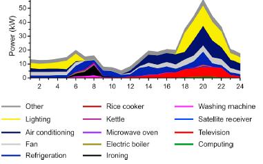
Figure 2. Hourly variation of appliance electricity consumption in 100 monitored households of Accra city for a typical A) weekday, B) Saturday and C) Sunday.

 

2.3 The Residential Appliance Consumption Model

In developing the residential appliance consumption model, a sub-model is designed to show the different functions and the datasets used for the sub-models. In the first instance, a regional household sample is selected to serve as a model for giving rise to the electricity consumption profiles of the city of Greater Accra, Ghana. Furthermore, a model is developed for home appliance ownership where the representative household sample is expected to be occupied with modern electrical appliances. Finally, a behavior model is used to develop the appliance behavior model’s outputs to replicate customer behavior metrics. Regarding this, the accumulated electricity consumption profiles are then simulated using the consumers’ appliance type as well as on the chosen appliance models and are simulated using the residents’ overall consumption profiles to determine the electricity demand trends of consumers.

 

For the first part of the model, a primary data representative sample of households in the Greater Accra Region, Ghana is selected to serve as a model for giving rise to electricity consumption profiles. For this study, there are specific conditions to be met: compressive, relevant information on the household level; such a sample is required for statistical analysis, permitting useful conclusions to be drawn and the residential model provides useful data on households which can be helpful for modeling appliance and ownership use. For the second part of the study, each household’s appliance demands must be captured as numbers and types of appliances as part of households in the survey. To achieve this, regional representative home appliance ownership was modeled using regional home appliance ownership statistics. The criteria used for the sample selection are: Home appliance ownership, the styles and number of appliances in the homes obtained at the chosen household level and a sizable sample to enable statistical evaluation and A regional representative sample. Following the previous literature reviewed, it is clear that the dataset satisfies the above criteria. To create a stochastic residential appliance consumption model for individual households, information like individual appliance usage habits, how and when consumers use appliances, is needed for the third component of the model, the appliance behaviour model. The criteria for selecting a sample to infer this data and algorithm the model are as follows: Detailed information on individual appliance uses for a multi-stage stochastic model; A high-resolution dataset for simulation and Identifying switch-on times, frequency and length of appliance usage, and power consumption profiles of individual appliances. A sizable sample to enable statistical evaluation, a regional representative sample and a household composition similar to the national dataset, as the home appliance ownership, depends on the household characteristics.

 

The residential household survey dataset fulfilled the research criteria by analyzing data from 100 households and about 1007 individual household electrical appliances. The tracked data includes accurate data of different electrical appliances used in the selected homes, and consumption data over a duration (one year) allows a look into how a household deals with the different appliances. Several computer programming languages and software methods have been used to build the stochastic demand model for the trend analysis. Anaconda software especially the RStudio and MATLAB are used to define indicators of customer behaviour, analyze the dataset for the chosen home appliances and examine the impact of appliance use on the household dataset. The model (household types, appliance ownership, and electricity demand) has been introduced in the MATLAB language. The multi-stage stochastic method is introduced in MATLAB by using the stochastic simulation kit random number generator in MATLAB. The 2-minute appliance power data were cleaned prior to analysis. Identifying bad readings in time series plots was done with a visual assessment. Roughly 0.06% of the values were deemed inaccurate, and they were discarded from the data set. To avoid skewing data based on the daily user activity, the whole day was erased when a substantial part of it was absent. When there were gaps in the data (of up to 4min each), they were filled in by applying linear interpolation to estimate the values. This technique was used to estimate around 0.002% of the data. The fact that data cleaning changes only affect a limited number of total readings implies that the influence on the analysis and outcomes should be negligible.

 

2.3.1 Household Characteristic Survey

The household questionnaire survey is a regional survey conducted by the researchers to gather information about people’s housing conditions, as well as the state and energy quality of housing in Greater Accra, Ghana. The project employs a dynamic multi-stage approach comprised of two major components: an initial interview survey of selected homes, followed by a physical examination of a sub-sample of around 100 of these households. Each household’s interviews were consolidated into a database. The dataset contains variables per home on income, household characteristics, tenure, electricity use, identity, second homes. To standardize the results, weighting factors are used. Weighting methodology includes a series of steps that consider selection and response processes involved in research. There was a Follow-Up Survey was conducted for appliance owner surveys by the researchers. The follow-up analysis was undertaken to soften the blow from the initial study. The project was financed by the researchers and data were obtained from 100 households through face-to-face surveys and from households chosen for their electricity use via the implementation of electricity monitors. The Residential Household Follow-Up Survey was used to collect 15 variables per home, including refrigerator possession, cooking and appliance use, hot water consumption, ventilation, lighting, tariffs, and many more. Interviews from each house were gathered into a database that could be used for demand response. Therefore, the results presented from the demand response residential household Follow-Up Survey reports are representative of the Ghana Residential Energy Use and Home appliance ownership Survey conducted in 2012 by the Energy Commission. Interviews from each house were gathered into a database that could be used for demand response.

 

The links to the household electricity consumption dataset were provided by the electricity company of Ghana in terms of individual household bill records. There was a complete record of each household’s behaviour in a database. The variables that were monitored and collected in the household electricity consumption are electricity use on daily basis, appliance characteristics, demographics and household characteristics, electricity rating, and details of house types. The electricity demand dataset is further split into many more files. The appliances are arranged using codes, with detailed points alongside the electricity demand of the individual appliances which is determined with a minute elapsed time and resolution. Table 4 estimation indicates the number of various appliance types in the household. Every single one of the 1,615 appliances in the home was monitored.

 

Table 4. Household Electricity Consumption of Appliances Monitored

 

Two distinct groups of samples were picked. The first community was private households/owner-occupied (no more than four occupants) and compound settlement communities in Accra with four and above inhabitants. Figure 3 shows the location of the private buildings. Between 1990 and 2015 all the houses were designed in styles by various developers. Figure 4 shows the various styles of houses in the East Legon neighbourhood of Accra and at different positions and sizes of houses. The East Legon neighborhood has been chosen to investigate the effect of consumer behaviour change on a specific residential feeder, where most houses are linked to prepaid meters (smart meters). The East Legon neighbourhood is one of the most affluent and attractive residential areas in Accra, north-east of central Accra, 10min from Accra Mall, 20min from Kotoka International Airport, and bordering the Tema motorway, Spintex, and the Legon-Madina highway. East Legon boasts beautiful residential and industrial buildings as well as a rapidly increasing industrial fringe, showcasing what was once Ghana’s first shopping mall, the A&C shopping center, a drive-through KFC, various banks along Lagos Avenue, several hotels, and many restaurants with excellent food for the area’s highly multicultural residents. Life in East Legon entails two big downsides. One is that the water supply is unreliable, forcing most people to either install a borehole. Second, while electricity supply is a known problem in Accra, East Legon is one area with very no known erratic, intermittent, and long blackouts that get the short end of the stick because many residents have power generators. The field was selected so that the network company’s real power demand data could be used for the subsequent request-response study. There were about 2400 households linked to the national grid in 2018[45].

 

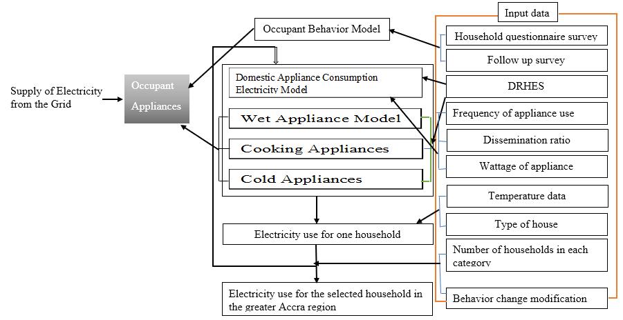
Figure 3. Agent-based appliance model development outline[46].

 

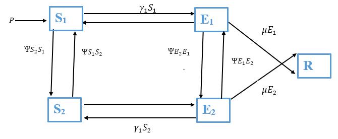
Figure 4. Schematic representation of the consumption reduction model.

 

The second category was randomly chosen households around the East Legon city area in representative neighborhoods. Such houses were chosen for equal representation of the general property of Accra households. Table 5 shows the relative positions of the areas where the survey was carried out. In total, it picked 500 households. This number consisted of a combination of old houses constructed in the 1970s with postpaid meters, fairly new houses, small and large houses, townhouses, and so on. The participants completed and returned a total of 200 out of the 500 questionnaires provided, reflecting a response rate of 40%.

 

Table 5. The Survey Objective, Sample Size, and Response Rates

 

In the different households, the age of the households is again restricted to the age of the user who has replied to the questionnaire. Reports using the household survey data collection for demand responses do not take gender into account. Only the households’ working condition, such as unemployed, pensioned and paying full-time, is known about earnings and jobs. The appliance electricity consumption dataset is shown in Figure 2. The column indicates the power in Kilowatt; the row shows the appliance type.

 

2.3.2 Synopsis of the Domestic Appliance Consumption Model

In developing the agent-based appliance model, a sub-model is designed to show the different functions and the datasets used for the sub-models. In the first instance, a regional household sample is selected to serve as a model for giving rise to the electricity consumption profiles of the city of Greater Accra, Ghana. Furthermore, a model is developed for home appliance ownership where the representative household sample is expected to be occupied with modern electrical appliances. Finally, a behaviour model is developed where consumers behaviour metrics are simulated using the results of the appliance behaviour model. Regarding this, the accumulated electricity consumption profiles are then simulated using the consumers’ appliance type as well as on the chosen appliance models and are simulated using the residents’ overall consumption profiles to determine the electricity demands as can be seen in Figure 3.

 

For the first part of the model, a primary household data representative sample of households in the Greater Accra Region, Ghana is selected to serve as a model for giving rise to electricity consumption profiles. In order to choose this study, there are specific conditions to be met: compressive, relevant information on the level household. Such a sample is required for statistical analysis, permitting useful conclusions to be drawn. The residential model provides useful data on households which can help model appliance and possession use.

 

The 2019-2021 demand response residential household dataset fulfills the requirements listed above is fairly accurate, detailed, up-to-date, and covers all housing conditions in Ghana. For example, houses were randomly chosen in the demand-side household survey to obtain a representative sample of residences in Ghana. An appendix of further response to the data year, demand residential household survey can be found below.

 

For the second part of the study, each household’s appliance demands must be captured as numbers and types of appliances as part of households in the survey. To achieve this, regional representative home appliance ownership will be modeled using regional home appliance ownership statistics. The criteria for selecting a sample to represent the home appliance ownership model are as follows:

Home appliance ownership: the styles and number of appliances in the homes obtained at the chosen household level.

A sizable sample to enable statistical evaluation.

A regional representative sample.

 

Following the previous literature analysis, it is clear that the 2019-2021 dataset satisfies the above criteria.

 

To create a stochastic agent-based appliance model for individual households, information like individual appliance usage habits, how and when consumers use appliances, is needed for the third component of the model, the appliance behaviour model. The criteria for selecting a sample to infer this data and algorithm the agent-based appliance model are as follows:

Detailed information on individual appliance uses for a multi-stage stochastic model.

A high-resolution dataset for simulation.

Identifying switch-on times, frequency and length of appliance usage, and power consumption profiles of individual appliances.

A sizable sample to enable statistical evaluation.

A regional representative sample.

A household composition similar to the national dataset, as the home appliance ownership, depends on the household characteristics.

 

The 2019-2021 demand response residential household survey dataset fulfilled the research criteria by analyzing data from 100 households and about 1007 individual household electrical appliances. The tracked data includes accurate data of different electrical appliances used in Ghanaian homes, up-to-date and high-resolution software for simulation. Collecting consumption data over a duration (one year) allows a peek into how a household deal with numerous appliances. However, the dataset is disputed by some who claim it does not reflect all Ghana households. Several computer programming languages and software methods are being used to build the stochastic transportation demand model. Anaconda software such as RStudio, JupyterLab, Qt Console, Spyder, and MATLAB are used to define indicators of customer behaviour, analyze the dataset for home appliance ownership from the household dataset and examine the impact of appliance use on the household dataset.

 

2.3.2.1 Demand Response Mathematical Model of Reduction in Consumption Using ODE

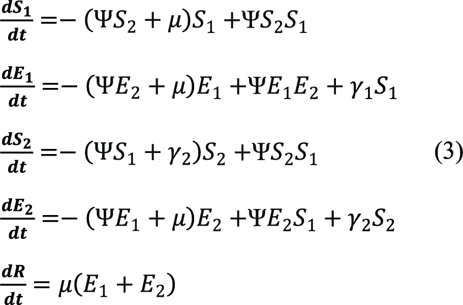
The agent-based model captures realistic individual-level behavior patterns and coordinated reactive changes in human behavior in order to better predict the reduction dynamics of consumption of electricity in residential homes. In our ODE model, the population is divided into two subgroups: a group that does not change its behavior or has normal behavior (subscript 1) and a group that modifies its behavior in response to a piece of available information (subscript 2). People move back and forth between the two groups (reducing consumption) depending on the behavior adopted. Individuals in each activity group are characterized by their behavioral status: the population of consumers that can reduce electricity S1 and E1 population ready to reduce due to certain behavior modification/information provision, while the second group population is also subdivided into consumers who are liable to be influenced by certain behavior changes S2, consumers who do not show any interest in the reduction of electricity E2 and R consumers who show signs of electricity reduction after introduction of behavior modification in households as shown diagrammatically in Figure 5. Because we are primarily interested in the effectiveness of changes in behavior for different appliance types, we use an open system with movement in or out of the population. Thus,

 

 

It is assumed that a certain fraction of the population will change their behavior to bring about reduction or reduce their consumption level. Let ΨS2S1 and ΨE2E1 be the consumption rates from the S2 and E1 classes to the S2 and E2 classes, respectively, and ΨS1S2 and ΨE1E2 be the consumption rates from the S2 and E2 classes to the S1 and E1 classes, respectively. The consumption rate coefficients are modeled by step functions given by:

 

 

For i=S1, E1, S2 and E2, where the parameter C is a positive constant that determines the rate of movement and τ is the time that determines when the new behavior is adopted.

 

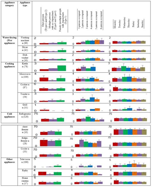
Figure 5. The number of times appliance is used per day per home, number of inhabitants, and day of the week.

 

Using the transfer diagrams in Figure 4, we obtain the following system of differential equations:

 

Schematic relationship between people who adopt a new behavior in response to the needed provision of reduction information and people who do not change their behavior. The arrows that connect the boxed groups represent the movement of individuals within the households. Households who are ready to adapt to new behavior in response (S1 or S2), people who do not change their behavior (E1 or E2) at rates γ1 or γ2; people who do not change their behavior at a rate μ; and people change their behavior based on the rates ΨS2 , ΨE1 , ΨS1, or ΨE2:

 

 

Where γ1 (for normal behavior) and γ2 (for modified behavior) are the forces of reduction. γ1 and γ2 incorporate the probability of appliance use, α, the reduced number of appliances because of indicative reduction, β, and 1-φj (j=s or i), which accounts for the effectiveness of the behavior in reducing either consumption (φs) or no consumption (φi). α is defined as the consumption of the population multiplied by no consumption multiplied by the average number of appliances an individual has per day. The forces of reduction for both groups are shown by:

 

 

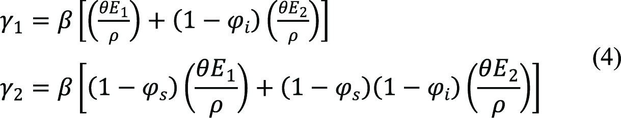
Where ρ=N-(1-θ) (E1+E2) and N is the total population N(t)=S1+E1+S2+E2+S3+R. In the forces of reduction, φi is incorporated into the reduction fractions because individuals in the E2 the class have adopted a new behavior and φs is incorporated into the reduction fractions in γ2 because individuals in the susceptible class (S2) have also adopted a new behavior. These forces of reduction and appropriate initial conditions complete our model formulation.

 

2.3.2.2 The Agent-based Model

The OPPIE simulation platform is an agent-based model that combines the demographic-based population of a region, a network of specific business and home locations, and the movement of individuals between locations with daily schedules. We simulated the consumption of electricity in households with different appliances using a synthetic population constructed to statistically match the 2010 Ghana Census population demographics of the Greater Accra region at the census tract level. This population only represents individuals reported as household residents; thus, visiting tourists, guests in hotels, and travelers in airports are not explicitly included. Each individual has a schedule of activities based on the Household Survey. A schedule specifies the type of activity, the starting and ending time, and the location of each assigned activity based on the type of appliances. The time, duration, and location of activities determine which individuals mix at the same location at the same time, which is relevant for demand response.

 

2.3.2.3 Model Assumption

The model to be formulated considers the following assumptions:

1. Individuals in self-apartments are considered as owners and individuals in rental apartments are considered as tenants.

2. The population considered is an open population.

3. Consumers in tenants are more ready to reduce.

4. Consumers in rental apartments can reduce electricity just as the owners.

5. Self-apartment consumers are assumed not to be bothered about the reduction in electricity in residential facilities.

6. Both individuals have an equal chance to reduce for all subpopulations.

 

2.3.2.4 The Mathematical Formulation of Model Parameters in MATLAB

According to Zhang et al.[47], there are eight stochastic demand response models considering different weights, decomposition approaches, and indicators. To decompose absolute electricity consumption change, which is quantity indicators, and discuss the results at the subcategory level, we apply additive decomposition analysis in this thesis. The total electricity consumption in the residential sector in year t is Yt, and it can be expressed as follows:

 

 

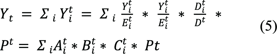
where, Yti,Eti,and Dti,represent the total electricity consumption, Household Electricity Consumption of Appliances and Demand Response Household Electricity Consumption, respectively, of residential sector i in year t. Dt is the household dataset in year t and is the total active households surveyed year. denotes the share of the residential electricity consumption to the total electricity consumption after the consumer behaviour changes of i in year t; is the Household Electricity Consumption of Appliances of i in year t and is the household structure. The electricity consumption increases from a base month of 0 to a target month t is represented by ΔYtρ.It can be resolved into five influencing drivers:

(1) The change of the residential electricity consumption to the total electricity consumption to share an effect (ΔYtcs);

(2) The change of Household Electricity Consumption of Appliances intensity effect (ΔYtai);

(3) The change of household structure effect (ΔYts)

(4) The change of consumer behaviour activity effect (ΔYtcb). So, ΔYtρ can be calculated in the following formula:

 

The influencing factor in Equation (6) can be expressed as follows:

 

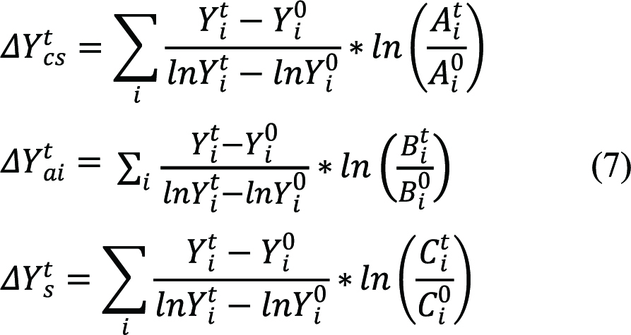
The electricity share indicates the effect of electricity consumption share in total consumption change in the change in behaviour. The electricity intensity evaluates the effect of demand response and efficiency improvement. The household structure denotes the influence of the residential structure adjustment on electricity consumption. The switch-on activities represent the effect of consumer behaviour on electricity consumption.

 

2.4 Analysis of Electricity Consumption Trends

2.4.1 Switch-on Events Measured

For each of the appliances in the housing electricity survey dataset, the average number of switch-on events was estimated by the methodology and description provided in Section 4. Table 6 demonstrates the summary figures on how many occasions a light switch was switched on by tenants for the 100 residential facilities. For washing machines, for example, the average number of switch-on events per day is calculated by dividing the total number of switch-on events by the number of days monitored. The average number of times a device is switched on every day is then determined by dividing the average number of times the system is switched on each day by the number of households. For device types, cold appliances have the most switches switched on, with a mean of 0.82 switches turned on every day depending on the 191 cold appliances in the dataset. Washing/drying appliances have the lowest number of switch-on incidents on a normal day. Fridge-freezers are the gadget seen at the highest level of being turned on, with an estimated regular number of cycles of 36.2 times a day. The findings demonstrate the systemic heterogeneity that occurs among all appliance forms. The findings reveal that one fridge-freezer had an average of 99.3 times on/off events per day during its testing duration, while another has an average of 3.5 times on/off events per day (the lowest observed). In addition to the frequent flipping on and off of the fridge-freezers during the day, this is triggered. According to the results, one chest freezer has an average of 99.3 events per day in their recorded period, while another chest freezer has an average of 5.5 events per day (the lowest observed). The home cinema had an average of 4.6 switch-on events a day and another home cinema has just 0.01 switch-on events over the whole tracking duration (the lowest observed). Ovens don’t have the largest number of regular on/off-hours, but they use the least number of on/off times every day.

 

Table 6. Statistics on the Total Number of Instances Appliance Types are Switch on Per Day in the 100 Homes in the Dataset

 

2.4.2 Number of Switch-on Events for Consumer Numbers, Household Types, and Different Days

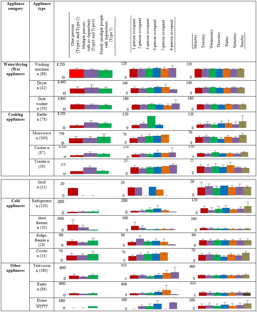
Figure 6 shows the average number of switch-on events each day for each appliance type, as well as their confidence periods, for various days of the week, occupant counts, and household types. In terms of the average regular number of switch-on incidents, there is no variance of the results across the week. It is impossible to speculate about how people with and without the appliances differ when the sample range is limited and nil where the appliances are not present in any of the homes, inhabitants, and day parties.

 

Different appliances were checked like the microwave, grill, and television. To show if there are substantial variations, one-way ANOVA was carried out. Given the occupant number, household form, and day forms, to calculate the mean value for the number of switch-on events each day, a one-way ANOVA test was used. Tables of the P-value of Levene’s test for the hypothesis of equivalent variance and p-value of ANOVA test are addressed in depth using the Levene’s test. Levene’s test findings indicate that for dishwashers there is a substantial impact of household form on the mean of the average amount of switch-on events each day at the P<0.05. There is considerable variance in the number of switch-on activities each day by the number of inhabitants at a house. For upright freezers, ANOVA reveals that there is a major impact of occupant number on switching on time at the P<0.05 mark. For the remaining appliances, ANOVA findings indicate that the total amount of switch-on activities each day is not substantially impacted by household forms, resident numbers, and what type of days. For purposes of the study, the data was not equally split between separate categories.

 

Figure 6. The mean of the number of actions a day that can be initiated is shown for the seasonality component.

 

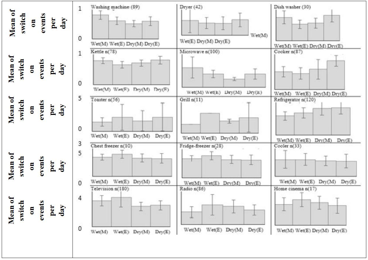
2.4.3 The Number of Switch-on Activities in a Season

In Figure 6, the mean and extent of the total number of switch-on events each day for each of the 15 appliances are estimated for the seasons: wet(M), wet(E), dry(M), and dry(E). The mean average amount of switch-on events per day is estimated, both monthly monitored households and year monitored households were used to measure the average number of switch-on activities per day. Due to a lack of evidence in certain seasons for the household electricity survey, some items of appliances could not be seen clearly in the graphs.

 

A one-way study of variation was performed on the means of the average amount of switch-on events each day during various seasons. The tables of P-values for Levene’s test and the ANOVA chart are included in the presentation. Only in the laundry machine, there’s a major impact of seasonality on the total regular amount of flipping on events at the P<0.05. When reviewing the data on the majority of the appliances, we found that there was no substantial change in the average regular number of switch-on activities during the spring or the fall. It demonstrates that inhabitants’ behaviors do not shift according to the season, even while preparing meals. The adjustment in the number of wash cycles for a washing machine is in proportion to the shifting seasons. More laundry may be cleaned in a continuous cycle as they become thinner, which helps in fewer occasions of the washing machines needing to be turned on.

 

2.4.3.1 Daily Number of Appliances Uses

The likelihood of triggering a switch-on event for each appliance from each day is shown in Figure 7. The findings in Table 7 differ from those in Figure 6 in that the number of switch-on activities for all 100 homes is seen each day. For example, the cumulative density frequency of washing machines is composed of 1567 points taken from the 62 households, and the likelihood of the number of switch-on events each day is seen for different numbers. The cumulative density frequencies graphs are useful for displaying the disparity in the number of days it takes to turn on, but they can’t reveal the variation in the number of times it takes to switch on. The cumulative density frequency in Figure 6 indicates the difference in the regular number of switch-on events found across all device forms across the dataset with certain days recording little use of the appliance and other days documenting multiple switch-on events. For example, approximately 80% of the days observed lacked the use of an oven while all cold appliances were used on at least one day during the observation era (lowest observed). The cool appliances recorded the largest number of switch-on in a day, and the fridge had the highest number of switch-on incidents in a day. This happens because the compressor continuously cycles as it works all over the day.

 

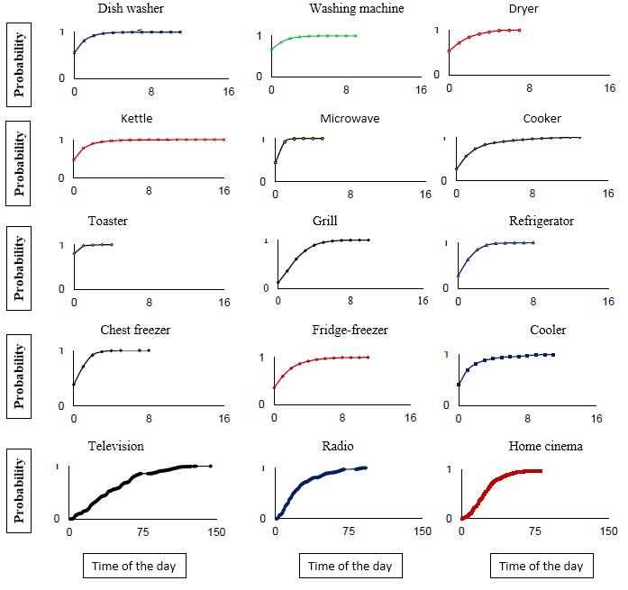
Figure 7. Daily cumulative distribution frequency uses of 15 appliance types.

 

Table 7. Switch-on Period Probabilities Across Different Household Types and Inhabitants

 

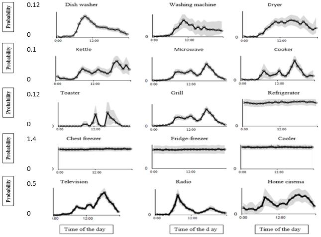
2.4.3.2 Analysis of Times for Daily Profiles of Switch-on Events

Figure 8 below depicts the related chance distributions for mean hourly switch-on times for the 15 appliance forms. The output of a production profile was measured from hourly time slots to show the overall pattern of the profile. However, for the model, the findings are obtained with two-minute odds. The points on the graph indicate how likely it is that you turn the light on over time. The findings indicate the varying periods it takes to turn on various forms of appliances. The number reflects the varied use of the equipment at various times in the day. Cooking machines are turned on at breakfast, lunch, and dinner hours. The peak period for running an automatic dishwasher is usually observed during the evening meal, while the peak time for running an automatic washing machine is typically observed in the morning. Cold machines are switched on periodically during the day. Televisions are turned on in the early morning and evening as well as in the middle of the day.

 

Figure 8. For each appliance form, the probability of the number of switch-on events (y-axis) versus the time of day (x-axis) is plotted.

 

2.4.3.3 Switch-on Period Probabilities Across Different Household Types, Inhabitant Numbers, and Days of The Week

The effects of the switch-on probabilities were meant for various forms of households and the number of inhabitants. However, inadequate data is crucial which defines how many groups there are. Therefore, in this segment, three categories were built to evaluate the distinction between one individual household (Type 1 and Type 2) two or more person households (Type 3 and Type 4), and family households (Type 5) for weekdays and weekends based on the literature. The household forms are clustered to account for a lack of details and are grouped into these three categories. The table indicates how many homes were used to calculate the average probabilities of switch-on times each day as can be seen in Table 7.

 

Figure 9 below demonstrates the possibility of each household type getting the various mean switch-on times during the day. This profile is determined by aggregating the hours of each employee, but not their actual results. The aim of creating these graphs is to compare; firstly, the probability of mean hourly switch-on times differing over weekday and weekends for each household group; secondly, for weekdays and weekends, the chance of mean hourly switch-on times for household groups was compared. Examples from each appliance group are listed and weighed against each other. Figure 8 suggests that there is no major variation in the form of the profile between household forms. In other words, the peak period as a percentage of the total number of switch-on occurrences for household appliances ranges based on the household form. The most frequent time of day for the starting of a washing machine spinning period is in the morning from 9am and 11am for single individual households. The prime period of the laundry machine turning on inside a household should not vary from 9am to 11am for several individuals and families. The figure indicates that the distribution of aggregate demand assumes the same form across weekdays and weekends. It indicates that the peak hours of appliance use are identical. For instance, the radio switching on odds is randomly distributed; weekday and weekend profiles are not distinctively different from each other. Most appliances stay at a steady temperature during the day regardless of the day of the week. Other appliance forms that are not shown have similar patterns to those shown in this analysis.

 

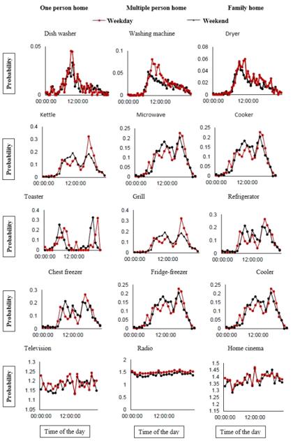
Figure 9. Comparative analysis of probability profiles of switch-on appliances on weekday and weekend daily times of the day.

 

2.4.3.4 Appliances Run Time

With each appliance in the dataset, the length of appliance use is determined using the option of appliance type model. Table 8 includes a description of the figures for the duration length of home rentals split down to peruse. By taking the average of the period per use for washing machines (60min for the first round, 30min for the second round, 15min for the third round: the average is (60+30+15)/3=35min of overall duration length per use for household number one). Then, the mean of the average number of events each day which is the average of the number of events per day for each household for the total number of households is determined. Television has the longest period of use per appliance, with the average user using the television for 230min per week. Next are Refrigerator (178.6min) and Laptop (14.6h) (175.8min). Grill had the shortest period per use, at a mean of 2.4min using the 30 video senders in the given dataset. After other appliances, cooking/cooling appliances are the appliance group with the second-highest average period length used per use in total based on the 372 cooking/cooling appliances in the dataset. The figures show that one grill runs for an average of 31.2min after it has been used (the highest observed in the dataset for grills).

 

Table 8. The Data Collected after the Reporting Cycle (Minutes) for Any Appliance for the Entire Monitoring Duration

 

2.4.4 Times for Household Types, Consumer Numbers, and with Different Days

Figure 10 displays the meantime (minutes) of events between appliances and household forms with their 95% confidence intervals of 100 homes plotted through different customer numbers, different days of the week. The statistics show that there is little difference between the households and the customers and that there are fewer consumers on Fridays than on any other day. It has proven difficult, however, to determine the number of customers as we only have a few respondents. This involves cooking appliances such as microwaves (100), toasters (78), and cookers (180). A one-way analysis of variance was used to determine the influence of household type, customer number, and day forms on the average number of switch-on occurrences each day. A resource with further information about. The ANOVA results indicate that there is no statistically significant difference across household kinds, occupant counts, or day types. As a result, there is no reason to distinguish the period distributions of subgroups at various phases.

 

Figure 10. Average duration length per use across different household types, consumer numbers, and day of the week.

 

2.4.4.1 The Durations for Different Time Slots

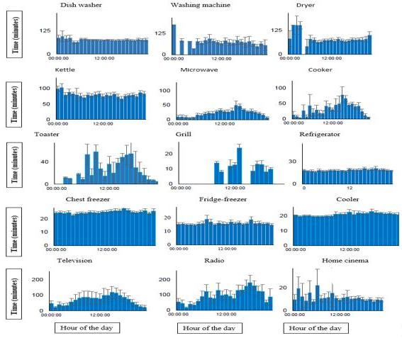
Figure 11 displays the total time of a specific appliance with the 95% confidence interval that the appliance was used throughout the particular span (on the y-axis). In the example, the switch-on events of all 100 households were grouped at 14:00 and 14:25. Next, the average period for each hour was determined, for shift lengths of any duration. One-way ANOVA is used to determine whether there are major differences in the results. The null hypothesis that variances are equal should be rejected according to the ANOVA test. Finally, it was determined that there is a time (minutes) difference between time-slots for both TV, radio, home theatre, laptop, and cooking appliances (Kettle, microwave, cooker, toaster, oven, grill). Consumers use television and cooking appliances longer in the evening and show it is used more during the nighttime. This may have an effect on the model’s results, which will be addressed further in the next section. The figure shows significant variation in duration for the different appliances between the amount of time spent on wet, cold, or electric equipment between the time slot.

 

Figure 11. Average of the times of appliance activities within 95% confidence interval that starts in the time interval.

 

2.4.4.2 Time of Each Use

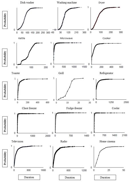
The average distributions of the period and length of how long appliances are used over time are shown in Figure 12. These results are different from Table 8 in that the time length for use is shown, which is Step 3 in the user data, instead of the average time length for a use per household. For example, for the cumulative density function of washing machines, data is taken from 62 households and cycles of washing machines lasting from 2 to 180min. The cumulative density function graphs are important to show the degree of variation in the time between different use within the same household. The graphs indicate that various appliances are used for different durations per day in the residential dataset. Coolers have a poor average storage duration of between 1min and 30min. In one day, the television was on for over 13h (the largest found was televisions in the dataset). The lifespan of these coolers varies considerably, but those that last for long periods tend to be on for long periods. The length of time used by appliances during use was less than 240min, with more than 60% being less than 90min. The length of the washing machine cycle varying from 10min to 0.5h.

 

Figure 12. Analysis of the total distribution of period length of 15 appliances and how they are used.

 

3 DISCUSSION

The novelty of this paper explores new ideas related to the creation of household electrical appliance usage behavior models. This paper has added to the studies on residential appliance use in as was discussed earlier[48]. This research relies a lot on appliance-level power data to build the high-resolution stochastic model relative to previous studies that focus on daily data. The data tracked appliance electricity consumption of controlled households’ monthly averages for this study. This dataset has some benefits as opposed to previous research that used consumer daily electricity time and power demands for predetermined demands. In this strategy, the everyday movements of the people cannot be traced down to particular dates. From section 5.3, it can be concluded that appliance on/appliance turn-on and appliance on/appliance turn-off states can be tracked. Furthermore, Section 5.3.2 demonstrates that some appliances are less than 10min long-term such as cold appliances (3 to 6min), and others longer than 10min such as cold appliances (15 to 30min) and other appliances (3 to 18min). For this purpose, the residential dataset is best suited to classify these short events instead of the complete activities. The minimum monitoring period for the data was at least 28 days for the study, various electricity consumption patterns were found within the same household.

 

On the household records, a variety of appliance behaviour is identifiable. This is accomplished by generating independent probability density functions for on-times and cumulative distribution functions explained earlier. This indicates, however, that the observations are to some degree hindered by the brief monitoring time and small sample size. An example is that the homes were monitored between 15 and 40 days, during which the equipment was relocated to another residence. This was required to keep the measuring equipment at a minimum level that was essential for the survey. Households were detected during various observation times, with different appliances. If these differences in appliance behaviour are attributable to household characteristics, climate fluctuations, or other variables are confounding the results. Until recently, it has not been feasible to research how much electricity each appliance uses because the cost of allocating a smart plug was too high for consumers. These sensors cannot be used in a majority of individual appliances and households. Smart and wired homes have simpler and less expensive monitoring, increasing the amount of data available for potential surveys, and enabling studies to be run over long periods and with a larger number of households. This can help to understand the variety of dynamic causes that contribute to particular behaviors of different household styles at different periods.

 

The various behaviors of consumers were differentiated depending on the number of residents in the household and their economic status (i.e., married vs. unmarried, household pensioners, and so on). A limited consistency among households, for example, House 1 has two inhabitants, such as a grill and cooker; however, none of the other houses in the dataset have both. The demand response household electricity survey dataset could not be meaningfully compared in this instance. In the analysis, it is shown that the difference between the number of inhabitants and household forms cannot be assessed by an ANOVA. Several cooking appliances, such as grills (n=87) and ovens (n=40) and televisions (n=180) are also are part of this category. The separation of the sample into subsets can reduce the model’s predictive capability due to data scarcity. A significantly broader study would be advantageous to boost the sample coverage and to confirm the outcomes of the current study. Additionally, the residential data measured the quantity of electricity used by household equipment and not their inhabitants. Data had to be examined at the personal level, but not at the household level; since it was only difficult to determine who is in whose households an appliance was on when they were turned on, it had to be monitored in households. It is currently unclear if appliance consumption behaviors for individuals are inter-correlated or whether inter-related. Since the residential dataset measured the appliances’ electric demands rather than individuals’ actions, it was important to determine it from these measurements. for example, if the energy demand drops to zero, any use was inspected to make sure that the turn-on and turn-off periods were right. There was a total of 161 wet appliances that were tested for 28 days. Approximately 4,508 separate days were required to conduct the manual study. Modeling may be called slow since it takes a long time. Larger and more well-defined case studies are needed to fully validate models which consider differences in the sample (such as household size, number of residents, income, etc.).

 

4 CONCLUSION

4.1 Conclusion

In summary, residential power reduction is clearly a regenerative path with new economic thinking in areas such as technological advances, societal awareness (reducing supply inequality) and political drive, which is basically a young generation with a restructuring mindset builds to enable system transformation delivering demand-response and climate adaptation ambitions. Replacing investments in supply to meet demand with household behavioral changes in device use can reduce electricity consumption and supply inequality, among other things, but adopting a behavioral approach to mitigation actions leads to academic and social responsibility in sustainable mobility. We must never just look at the bottom line, we always need to look at the whole value chain and then reassess how green a climate friendly outcome actually is and the SDGs don’t limit their focus to the bottom line. They also consider social, human and natural impacts, as well as economic impacts on resource-supplying nations. We are in a global economic and energy transition. We need to change the way we see things by breaking free from the old iron-clad ways of thinking. We need to broaden our view, looking back, forward, up and down, to understand that Demand Response will be the way forward in the years to come. To ensure the successful implementation of a clean, fair and just energy transition that leaves no one behind requires leadership and representation from the private sector, with representatives from both working towards a common goal would be an interesting place to start.

 

4.2 Policy Implications

The findings of the present research work provides decision-makers with detailed information on the main factors influencing household electricity consumption and energy consumption patterns, which would enable them to improve policy frameworks, e.g. As a result, optimal package size design, improved technology decisions, and capacity decisions can be made. It would also allow home designers and HVAC engineers to better understand underlying sales growth and actual behavioral distribution. Utilization of building simulation tools is greatly increased through the detection and distribution of consumer behavior, which is also essential for improving the accuracy of energy performance modeling results.

 

The research also took into account the difficulties consumers have had in purchasing energy-efficient home appliances over the past decade. We have found that energy-efficient home appliances use the least amount of energy and still perform at the highest level. It has been found that studies on the barriers to energy efficient appliances are much more common in developed than in developing countries. Furthermore, the barriers to efficient devices in Western countries have been studied through the lens of behavioral economics, ignoring the practical economics approach, while such studies are lacking in developing markets like Ghana. Therefore, to estimate the effect of barriers on consumer purchasing behavior for a future study, we offer a model based on planned behavior theory and prospect theory. It suggests that the study examines how factors such as perceived product dangers, behavioral control, perceived personal discomfort, and price sensitivity alter the linear relationship between purchase intent and behavior.

 

Acknowledgements

Not applicable.

 

Conflicts of Interest

The authors declared no conflict of interest.

 

Author Contribution

All authors participated in the drafting and writing of the manuscript. All authors contributed to the manuscript and approved the final version.

 

Abbreviation List

SDG, Sustainable development goal

TPP, Thermal power plants

VRA, Volta River Authority

IPPs, Independent power producers

 

References

[1] Ghana. Energy Commission of Ghana. National Energy Statistics (2007-2016). Accessed 2022. Available at http://energycom.gov.gh/files/ENERGY_STATISTICS_2017.pdf

[2] Ghana. Energy Commission of Ghana. National Energy Statistics (2008-2017). Accessed 2022. Available at http://energycom.gov.gh/files/ENERGY_STATISTICS_2018_FINAL.pdf

[3] US. Center for Global Development. The Electricity Situation in Ghana: Challenges and Opportunities. Accessed 2022. Available at https://www.cgdev.org/sites/default/files/electricity-situation-ghana-challenges-and-opportunities.pdf

[4] Ghana. Energy Commission of Ghana. National Energy Statistics (2009-2020). Accessed 2022. Available at https://energycom.gov.gh/files/ENERGY_STATISTICS_2019.pdf  

[5] Sarkodie SA. Lessons to be learned from Ghana’s excess electricity shambles. Accessed 2022. Available at: https://theconversation.com/lessons-to-be-learnt-from-ghanas-excess-electricity-shambles-121257  

[6] Adom PK. Asymmetric impacts of the determinants of energy intensity in Nigeria. Energ Econ, 2015; 49: 570-580. DOI: 10.1016/j.eneco.2015.03.027

[7] ISSER. Electricity insecurity and its Impact on Micro and Small Businesses in Ghana. Electricity Insecurity and Its Impact on the Economy of Ghana. 2015.

[8] Ahmed Z, Akerib DS, Arrenberg S et al. Results from a low-energy analysis of the CDMS II germanium data. Phys Rev Lett, 2011; 106: 131302. DOI: 10.1103/physrevlett.106.131302

[9] Sarkodie SA, Adom PK. Determinants of energy consumption in Kenya: a NIPALS approach. Energy, 2018; 159: 696-705. DOI: 10.1016/j.energy.2018.06.195

[10] Creyts TT, Schoof CG. Drainage through subglacial water sheets. J Geophys Res-Earth, 2009; 114: F04008. DOI: 10.1029/2008jf001215

[11] Strbac G, Gan CK, Stanojevic V et al. Benefits of Advanced Smart Metering for Demand Response based Control of Distribution Networks. 2010.

[12] Gottwalt S, Ketter W, Block C et al. Demand side management-A simulation of household behavior under variable prices. Energ Policy, 2011; 39: 8163-8174. DOI: 10.1016/j.enpol.2011.10.016

[13] De Blécourt MJ. Load-shifting in a new perspective: Smart scheduling of smart household appliances using an Agent-Bsaed Modelling Approach [master’s thesis]. Delft, Netherlands:  Technical University of Delft; 2012.

[14] Nauges C, Wheeler SA. The complex relationship between households’ climate change concerns and their water and energy mitigation behaviour. Ecol Econ, 2017; 141: 87-94. DOI: 10.1016/j.ecolecon.2017.05.026

[15] Wicker P, Becken S. Conscientious VS. ambivalent consumers: Do concerns about energy availability and climate change influence consumer behaviour? Ecol Econ, 2013; 88: 41-48. DOI: 10.1016/j.ecolecon.2013.01.005

[16] Belaid F, Garcia T. Understanding the spectrum of residential energy-saving behaviours: French evidence using disaggregated data. Ecol Econ, 2016; 57: 204-214. DOI: 10.1016/j.eneco.2016.05.006

[17] Oberst CA, Schmitz H, Madlener R. Are prosumer households that much different? Evidence from stated residential energy consumption in Germany. Ecol Econ, 2019; 158: 101-115. DOI: 10.1016/j.ecolecon.2018.12.014

[18] Carbon Trust. Carbon footprints in the supply chain: the next step for business. Carbon Trust, 2006. Accessed 2022. Available at: https://www.carbontrust.com/zh/node/947

[19] Martínez-Montejo SA, Sheinbaum-Pardo C. The impact of energy efficiency standards on residential electricity consumption in Mexico. Energy Sustain Dev, 2016; 32: 50-61. DOI: 10.1016/j.esd.2016.02.010

[20] Pelletier C, Rogaume Y, Dieckhoff L et al. Effect of combustion technology and biogenic CO2 impact factor on global warming potential of wood-to-heat chains. Appl Energ, 2019; 235: 1381-1388. DOI: 10.1016/j.apenergy.2018.11.060

[21] Niemelä T, Levy K, Kosonen R et al. Cost-optimal renovation solutions to maximize environmental performance, indoor thermal conditions and productivity of office buildings in cold climate. Sustain Cities Soc, 2017; 32: 417-434. DOI: 10.1016/j.scs.2017.04.009

[22] Quaglione D, Cassetta E, Crociata A et al. Exploring additional determinants of energy-saving behaviour: The influence of individuals’ participation in cultural activities. Energ Policy, 2017; 108: 503-511. DOI: 10.1016/j.enpol.2017.06.030

[23] Levesque A, Pietzcker RC, Luderer G. Halving energy demand from buildings: The impact of low consumption practices. Technol Forecast Soc, 2019; 146: 253-266. DOI: 10.1016/j.techfore.2019.04.025

[24] Salom J, Widén J, Candanedo J et al. Understanding net zero energy buildings: evaluation of load matching and grid interaction indicators: Proceedings of building simulation-12th Conference of International Building Performance Simulation Association, Sydney, Australia, 14-16 November 2011.

[25] Ziegler F, Seim S, Verwiebe P et al. A Probabilistic Modelling Approach for Residential Load Profiles. Energy Reso, 2020; 1-28. DOI: 10.5281/zenodo.3689339

[26] Yu Z, Haghighat F, Fung BCM. Advances and challenges in building engineering and data mining applications for energy-efficient communities. Sustain Cities Soc, 2016; 25: 33-38. DOI: 10.1016/j.scs.2015.12.001

[27] Australia. Australian Energy Market Commission. International review of demand response mechanisms. Accessed 2022. Available at https://www.brattle.com/wp-content/uploads/2017/10/5887_aemc_report.pdf

[28] Yohanis YG, Mondol JD, Wright A et al. Real-life energy use in the UK: How occupancy and dwelling characteristics affect domestic electricity use. Energ Buildings, 2008; 40: 1053-1059. DOI: 10.1016/j.enbuild.2007.09.001

[29] Wiesmann D, Azevedo IL, Ferrão P et al. Residential electricity consumption in Portugal: Findings from top-down and bottom-up models. Energ Policy, 2011; 39: 2772-2779. DOI: 10.1016/j.enpol.2011.02.047

[30] Bedir M, Hasselaar E, Itard L. Determinants of electricity consumption in Dutch dwellings. Energ Buildings, 2013; 58: 194-207. DOI: 10.1016/j.enbuild.2012.10.016

[31] Halvorsen B, Larsen BM. The flexibility of household electricity demand over time. Resour Energy Econ, 2001; 23: 1-18. DOI: 10.1016/S0928-7655(00)00035-X

[32] Genjo K, Tanabe S, Matsumoto S et al. Relationship between possession of electric appliances and electricity for lighting and others in Japanese households. Energ Buildings, 2005; 37: 259-272. DOI: 10.1016/j.enbuild.2004.06.025

[33] Darby S. The effectiveness of feedback on energy consumption: A Review for DEFRA of the Literature on Metering, Billing and direct Displays. Oxford, UK: Environmental Change Institute, University of Oxford; 2006.

[34] Carlson DR, Matthews HS, Bergés M. One size does not fit all: Averaged data on household electricity is inadequate for residential energy policy and decisions. Energ Buildings, 2013; 64: 132-144. DOI: 10.1016/j.enbuild.2013.04.005

[35] Zhou S, Teng F. Estimation of urban residential electricity demand in China using household survey data. Energ Policy, 2013; 61: 394-402. DOI: 10.1016/j.enpol.2013.06.092

[36] He J, Young AN, Pathan A et al. Air conditioning Energy Use in Houses in Southern England: Proceeding of Dynamic Analysis, Simulation and Testing applied to the Energy and Environmental Performance of Buildings Conference, Athens, Greece, 12-14 October 2005.

[37] Kim Y, Son H, Kim S. Short term electricity load forecasting for institutional buildings. Energy Rep, 2019; 5: 1270-1280. DOI: 10.1016/j.egyr.2019.08.086

[38] Cogan D, Camilleri M, Isaacs N et al. National Database of Household Appliances-Understanding Baseload and Standby Power Use: Energy Efficiency in Domestic Appliances and Lighting (EEDAL) Conference, London, June, 2006.

[39] Yilmaz S. Stochastic bottom-up modelling of household appliance usage to quantify the demand response potential in UK residential sector [doctor’s thesis]. Loughborough, UK, Loughborough University; 2017.

[40] Gyamfi S. Demand Response Assessment and Modelling of Peak Electricity Demand in the Residential Sector: Information and Communcation Requirements [doctor’s thesis]. Christchurch, New Zealand, University of Canterbury; 2010.

[41] UK. Department of Energy and Climate Change. Household Electricity Survey. Available at https://www.gov.uk/government/publications/household-electricity-survey--2

[42] Leahy E, Lyons S. Energy use and appliance ownership in Ireland. Energ Policy, 2010; 38: 4265-4279. DOI: 10.1016/j.enpol.2010.03.056

[43] Ireland. The Economic and Social Research Institute. Electrical Appliance Ownership and Usage in Ireland. Accessed 2022. Available at http://www.tara.tcd.ie/bitstream/handle/2262/63755/WP421.pdf?sequence=1

[44] Sakah M, du Can SR, Diawuo FA et al. A study of appliance ownership and electricity consumption determinants in urban Ghanaian households. Sustain Cities Soc, 2019; 44: 559-581. DOI: 10.1016/j.scs.2018.10.019

[45] Salahuddin M, Alam K, Ozturk I et al. The effects of electricity consumption, economic growth, financial development and foreign direct investment on CO2 emissions in Kuwait. Renew Sust Energ Rev, 2018; 81: 2002-2010. DOI: 10.1016/j.rser.2017.06.009

[46] Qayyum FA. Appliance scheduling optimization with micro-grid in smart home network [master’s thesis]. Ryerson University. Toronto, Canada: Ryerson University, 2015. DOI: 10.32920/ryerson.14668311.v1

[47] Zhang X, Qin P, Hu N et al. Household Appliance Ownership and Income Inequality. In: Zheng X, Wei C ed. Household Energy Consumption in China: 2016 Report. Springer: Singapore, 2019; 195-217. DOI: 10.1007/978-981-13-7523-1_7

[48] Richmond J, Urpelainen J. Electrification and appliance ownership over time: Evidence from rural India. Energ Policy, 2019; 133: 110862. DOI: 10.1016/j.enpol.2019.06

 

Copyright ©2022 The Author(s). This open-access article is licensed under a Creative Commons Attribution 4.0 International License (https://creativecommons.org/licenses/by/4.0), which permits unrestricted use, sharing, adaptation, distribution, and reproduction in any medium, provided the original work is properly cited.