Estimation of the Parameters of the State of Agrocenoses Based on Remote Sensing Data

 

Ilya Mikhayilovich Mikhailenko1*

 

1Laboratory of Information Systems of Agrophysical Research Institute of the Russian, Academy of Sciences, St. Petersburg, Russia

 

*Correspondence to: Ilya Mikhayilovich Mikhailenko, PhD, Associate Professor, Laboratory of Information Systems of Agrophysical Research Institute of the Russian, Academy of Sciences, Grazhdanskiy Prospekt, St. Petersburg 195220, Russia; Email: ilya.mihailenko@yandex.ru

 

DOI: 10.53964/jmab.2022017

 

Abstract

Objective: The purpose of this study is to substantiate the method and means of forming estimates of the physical parameters of the state of agrocenoses, including the main agricultural crops and weeds. These physical parameters include biomass parameters, the estimates of which will be used to address the technological issues of future agriculture management.

 

Methods: With consideration of the differences in the physical dimension of information, a method for integrating ground-based measurements and earth remote sensing data is proposed by the joint use of a mathematical model of the dynamics of agrocenoses biomass state parameters and a model for the relationship between the calculated state parameters and remote sensing data. Spatial coordinates are the main feature of the mathematical models used, and the task of assessment is divided into the task of forming average field estimates of the parameters of the state of agrocenoses and their spatial correction for elementary sections of the field using a linear corrector.

 

Results: An algorithm for estimating the parameters of the state of agrocenosis according to remote sensing data was developed, which was implemented in a specialized computer program. Original sources of information were employed to ensure sufficient accuracy and reliability of the assessment. Ground measurements were used to identify and adapt mathematical models, including data from stationary remote sensing devices, and a mobile remote sensing tool was used to estimate the parameters of the biomass of agrocenoses over the entire area of the field.

 

Conclusion: The proposed method and the algorithm for its implementation ensure the stability of the estimation process with an error in assessing the biomass of agrocenoses being ±10%. The current research has been carried out over the past 10 years in the experimental fields of the Menkovsky branch of the Agrophysical Institute, within the framework of the thematic plan of the Agrophysical Institute in the scientific direction of "Precision Farming".

 

Keywords: agrocenoses, remote sensing, mathematical models

 

1 INTRODUCTION

The transition to digitalization and intellectualization of agriculture is primarily associated with the automation of agricultural technology management processes, which requires reliable information on the parameters of the state of crops and the degree of their contamination by weeds. Moreover, these parameters are the physical and chemical parameters of agrocenoses and the soil environment. Estimates of these parameters allow management to formulate control decisions and develop control instructions in automatic control systems.

 

The main problem with the assessment contains cultivated and weeded plants, and classical methods of assessment and pattern recognition are thus necessitated. Earth remote sensing (ERS) facilities are adopted to address these issues, in which various options for indices and optical criteria are frequently used. Specifically, the normalized difference vegetation index is mostly used. Its concept o was presented by Kriegler et al.[1], and was first described by Rouse et al.[2] This index has been transformed into various variants such as the relative vegetation index, first described by Jordan[3], differential growth index, first reported by Lillesand and Kiefer[4], and infrared growth index, first described Crippen[5]. In the information sense, the indices are scalar quantities obtained by combining the reflection parameters of individual spectral ranges[6-10]. Therefore, the use of indices is mainly associated with rough expert assessments of situations in the fields or with pattern recognition with simple dual alternatives, such as plant diseases, stresses, land classification, crop recognition, detection of phenological phases of crop development, and a generalized assessment of the state of crops of the “normal-abnormal” type. Nevertheless, such simple methods fail to solve the control problems in precision farming systems, To achieve the management goal, reliable quantitative estimates of the physical parameters of the state of crops and soil environment that determine the management goals are required.

 

In previous studies[11-14], an approach has been developed based on the classical estimation of the parameters of the state of crops according to remote sensing data and is considered an indirect measurement of the parameters of the state of the object of assessment. This approach has been tested on various forage crops whose biomass is a raw material for the preparation of forages. The present study aims to develop an approach to assess the parameters of the state of agrocenoses, which include cultivated plants with a more complex morphological structure and weeds of various species.

 

2 MATERIALS AND METHODS

The assessment of the parameters of the state of the agrocenoses is to construct in real-time estimates of such physical parameters as the density (amount of biomass per unit area) of a cultivated plant, including its commercial part (marketable yield), the density of the biomass of weed plants, as well as its composition of the total biomass by dry and wet mass. The estimates of these parameters are used for agricultural technology management. The classical approach to the estimation problem is to clarify a priori information about the estimated parameters by indirect measurements (remote sensing data in the current study), which is a source of a posteriori information about the parameters of the agrocenoses state.

 

All a priori information about the estimated parameters of the agrocenoses is contained in the mathematical model that reflects the dependence of these parameters on the main influencing factors. Herein, spring wheat was considered a cultivated plant.

 

Since the sowing of spring wheat has two different patterns, before heading and after its onset, two mathematical models were used in the estimation problem[11,12].

 

The detailed form of the model of biomass parameters of agrocenoses with spring wheat before the heading phase shows the following form[14]:

 

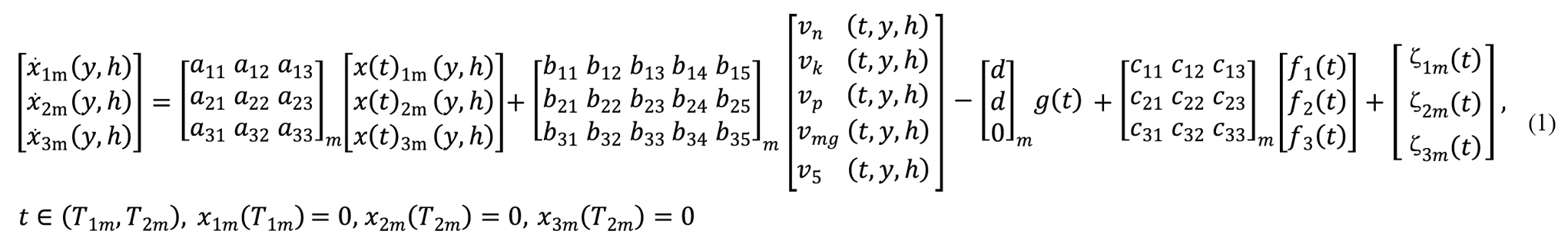
where the parameters of the state of the biomass of the agrocenoses are: x1m (y,h) is the density of the biomass of the cultivated plant on an elementary plot with spatial coordinates (y,h), hwt·ha-1; x2m(y,h) is the density of the biomass of weeds, hwt·ha-1; x3m(y,h) is the density of the wet mass of the agrocenoses, hwt·ha-1; external disturbances are: f1-average daily air temperature, C; f2-average daily radiation level, W·(m2·h.)-1; f3-average daily precipitation intensity, mm; parameters of the chemical state of the soil: vN-nitrogen content in the soil, kg·ha-1; vK-potassium content in soil, kg·ha-1; vP is the phosphorus content in the soil, kg·ha-1; vMg is the content of magnesium in the soil, kg·ha-1; v5-moisture content in the soil, mm; g is the dose of agrocenoses treatment with a universal herbicide, kg·ha-1;

 

-modeling errors, which are random processes with zero means and variances

 

y, h-spatial coordinates, m; t∈(T1m,T2m)-daily time, vegetation interval from germination to heading phase.

 

Vector-matrix symbolic form of the model (1)

 

where: Am, Bm, Dm, Cm are the matrices of model parameters, dynamic, transfer of control of chemical parameters of the soil, transfer of herbicide control, transfer of external disturbances, and the form of matrices corresponds to the expanded form of the model (1), Xm,V, F, Sm are the vectors of state parameters, nutrient content in the soil, climatic parameters, and random errors in modeling the model (1). The expanded form of the model of the parameters of the biomass of the agrocenoses with spring wheat after the beginning of earing has the following form[14]:

 

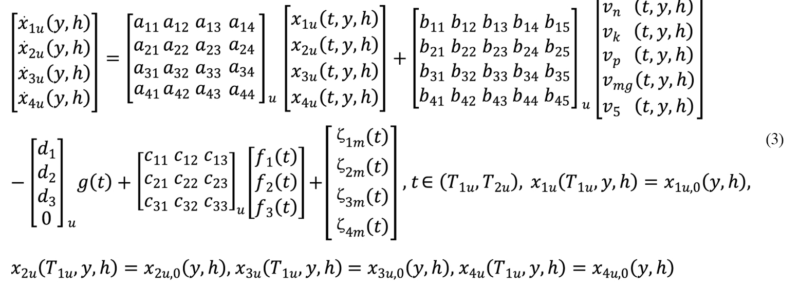
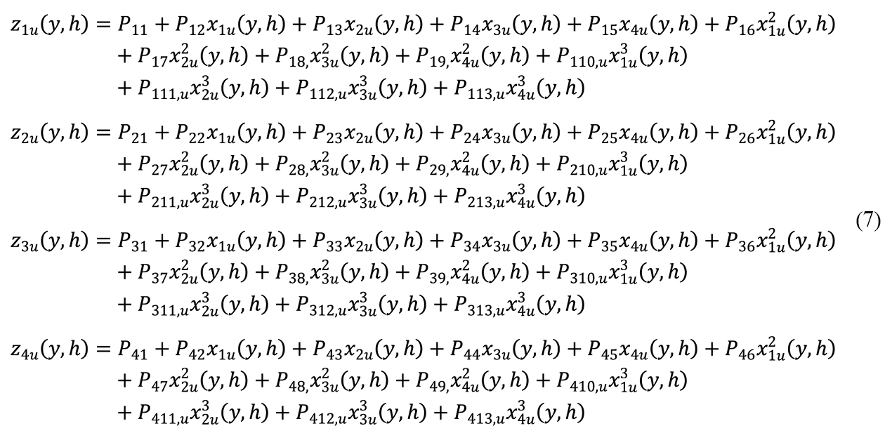
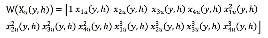
where the parameters of the state of the biomass of the agrocenoses are: x1u(y,h) is the density of the biomass of a cultivated plant (spring wheat) on an elementary plot with spatial coordinates (y,h), hwt·ha-1; x2u(y,h) is the density of biomass of weeds, hwt·ha-1; x3u(y,h) is the density of the mass of ears of spring wheat (yield), hwt·ha-1; x4u(y,h) is the density of the raw mass of the agrocenoses, hwt·ha-1;

 

-modeling errors, which are random processes with zero means and variances

 

y,h-spatial coordinates, m; -daily time, vegetation interval from the heading phase to the maturation phase.

 

Vector-matrix symbolic form of the model

 

where: Au, Bu, Du, Cu are the matrices of model parameters, dynamic, transfer of control of chemical parameters of the soil, transfer of herbicide control, transfer of external disturbances, the form of matrices corresponds to the expanded form of the model (3), Xu, V, F(t), Su are the vectors of state parameters, nutrient content in the soil, climatic parameters, and random errors in modeling the model (4).

 

A priori information on the parameters of the state of the biomass of the agrocenoses, formed by models (2), (4), should be corrected according to real ERS data, to which optical measurement models (ERS models) are introduced.

 

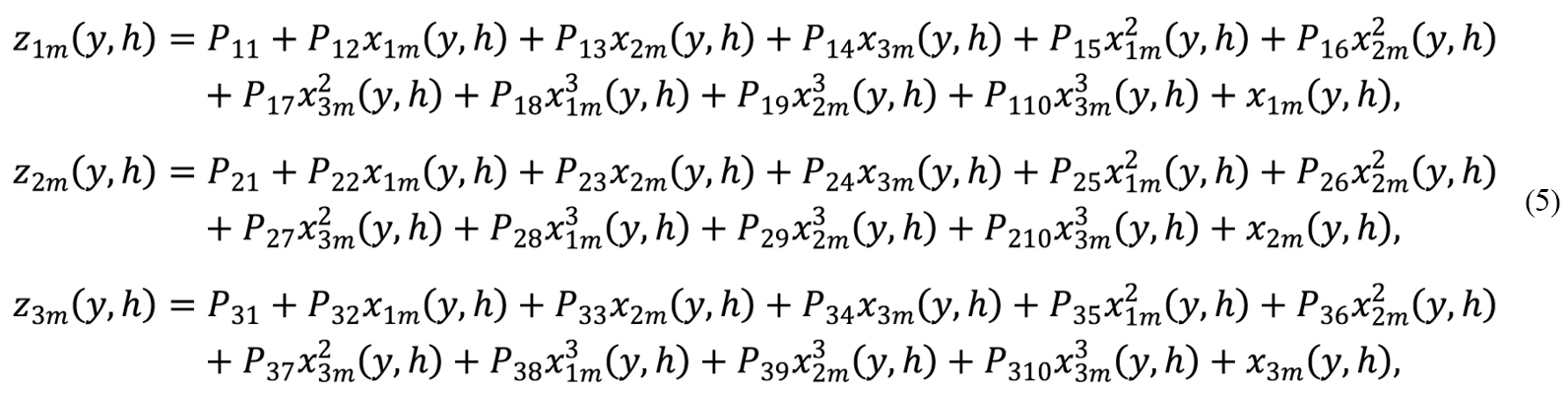
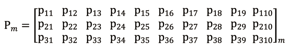
The model of optical measurements of the state of the biomass of spring wheat agrocenoses in the period preceding heading has the following form[14]:

 

symbolic vector-matrix form of the model:

 

where:

 

is the vector of reflection parameters for the spatial coordinate in the green range z1 (500-565nm), red z2 (625-680nm), (700-740nm) and near-IR range z3 (740-950nm)

 

-matrix of model parameters,

 

-vector-function, where the arguments are the parameters of the state of the agrocenoses; x1m, x2m, x3m8 are the random measurement errors with zero means and variances e2 1m, e2 2m, e2 3m.

 

Optical measurement model (ERS model) of the biomass state of agrocenosis with spring wheat for the period from the beginning of heading to crop ripening in an expanded scalar by-component form

 

symbolic vector-matrix form of the model

 

where:

 

-vector of integrated reflection parameters in green (500-565nm)-(z1m), in 1st red (625-700nm)-(z2m), in 2nd red (700-750nm)-(z2m), in the near IR (750-950nm)-(z3m),

 

-matrix of model parameters,

 

-vector-function, where the arguments are the parameters of the agrocenoses state.

 

The main feature of the presented vector-matrix mathematical models (1)-(8) is that the components of the vectors are not scalar or vector quantities but two-dimensional distributions of the corresponding biomass parameters in dynamic state models and reflection parameters in ERS models. Such models can be classified as a variety of 3D models, which significantly complicates the modeling and estimation algorithms and requires spatial cycles, where the number of variables depends on the method of dividing the total surface of the field into elementary sections. With an area of an elementary plot of 2m2, the number of computational evaluation cycles will reach 5000 for a field area of 1ha.

 

With a total area of the field under sowing of 500ha, the total number of elementary plots and algorithm cycles will be 2.5×106 units. Therefore, for large areas of crops (more than 1000ha), it is advisable to use approximate modeling and estimation schemes. In the estimation schemes, the parameters of the sowing state averaged over the field are estimated, followed by the correction of the estimates for the field surface using a corrective model without the indicators of the phenological state of the crop

 

 

where: K(t) is a matrix of spatial correctors, and its parameters are estimated by forming an array of variations in the reflection parameters of remote sensing ΔZ(t,y,h) and estimates of biomass parameters for 30-40 elementary sections for a given time t. Such points in time are only those in which technological operations are performed, while spatial corrector matrices are not established for the rest of the time points.

 

To form estimates of biomass parameters in the selected elementary areas, the following local estimation algorithm was used and built on the basis of the models (2), (4)[14,15]

 

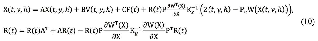
where: R(t) is the matrices of estimation errors, with the dimension corresponding to the vectors of the biomass parameters of the models (2), (4).

 

The estimation algorithm (10) implements the classical optimal filtering method[15]. The estimates generated by the algorithm (10) are used to form controls for the state parameters of agrocenoses. The components of this control are a sequence of fertilizer application rates, irrigation rates, and herbicide application rates. The formation of such departments is an independent problem that requires additional attention.

 

The reliability of estimates of parameters of agrocenoses generated by algorithm (10) depends on the accuracy of the mathematical models used (2), (4), (6), (8). It is achieved by the quality of their identification based on real data. This is availableonly when creating a special information-measuring complex, as shown in Figure 1.

 

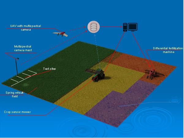
Figure 1. Functional diagram of the information-measuring complex for evaluating the parameters and managing the state of the agrocenoses.

 

It includes means of ground-based measurements and remote sensing of the ERS. The means of ground measurements include devices for measuring the parameters of the crop sowing biomass, weed biomass, and physical and chemical parameters of the soil environment. These funds were located on test sites, which were located at the edge of the field for easy maintenance. The number of such sites was 15-20 units, and the area of each site was 10-20m2. They were sown with the same crop as the main field with different doses of fertilizers, different irrigation rates, and varying degrees of weediness. Ground measurements include meteorological parameters meters located at the nearest weather station, which usually serves several fields.

 

ERS means include a stationary mast with a multispectral optical sounding device located above the test sites. In addition to the stationary device, the complex also includes a mobile remote sensing device based on an unmanned aerial vehicle (UAV). Ground-based measuring instruments and stationary remote sensing means were operated on a daily time scale and are used to identify mathematical models (2), (4), (6), (8). The mobile remote sensing tool functioned only on the days of technological operations and was used to form estimates of the parameters of agrocenoses using algorithms (9), (10).

 

To obtain experimental data, a UAV "Geoscan 401" equipped with a multispectral optical camera MikoSens RedH MX was used as a mobile remote sensing tool. Reflection parameters in the range from 430nm to 950nm were recorded using a multispectral camera over the entire area of the field with agrocenosis under spring wheat. A portable hyperspectrometer PSR+"Srectrora diameter" (USA), which is equipped with a built-in GPS system receiver, was used as a stationary remote sensing tool. The width of the optical range of the hyperspectrometer was 360-1350nm. A sampling of plant and soil biomass was carried out manually, followed by sample analysis in the analytical laboratory of the Agrophysical Institute. The institute's stationary weather station was used to collect data on climatic conditions.

 

All measurements were processed by the verification algorithm and recorded in the database and were introduced into the estimation algorithm (10). The received information is not subjected to any additional filtering, since the estimation algorithm (10) is an optimal filter, and random errors of meters and models are excluded[15]. The parameters of mathematical models (2), (4), (6), (8) are estimated by an independent identification algorithm operating on the principle of parameter control[15]. This algorithm minimizes the root-mean-square deviation of the vector of model state parameters from the real values of these parameters.

 

3 RESULTS

Figure 2 shows a fragment of remote sensing data of an experimental field with the sowing of spring wheat at the stage of milky-wax ripeness (green color). Test sites are highlighted herein, and soil is collected daily, from which information on the parameters of the state of agriculture is formed according to models (2), (4). While sampling by stationary ERS means, the daily average parameters of reflection over the test sites in the above spectral ranges were recorded. The obtained daily data were used to identify models (2), (4), (6), (8). The starting point for assessing the state of agrocenoses is the quality of models (6), (8). Graphs of the processes of identification of these models are presented in Figure 3.

 

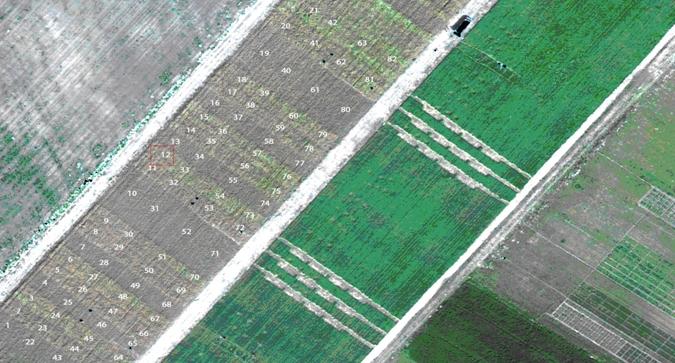
Figure 2. Image of an experimental field with sowing of spring wheat at the stage of milky-wax ripeness. Menkovsky branch of the Agrophysical Institute.

 

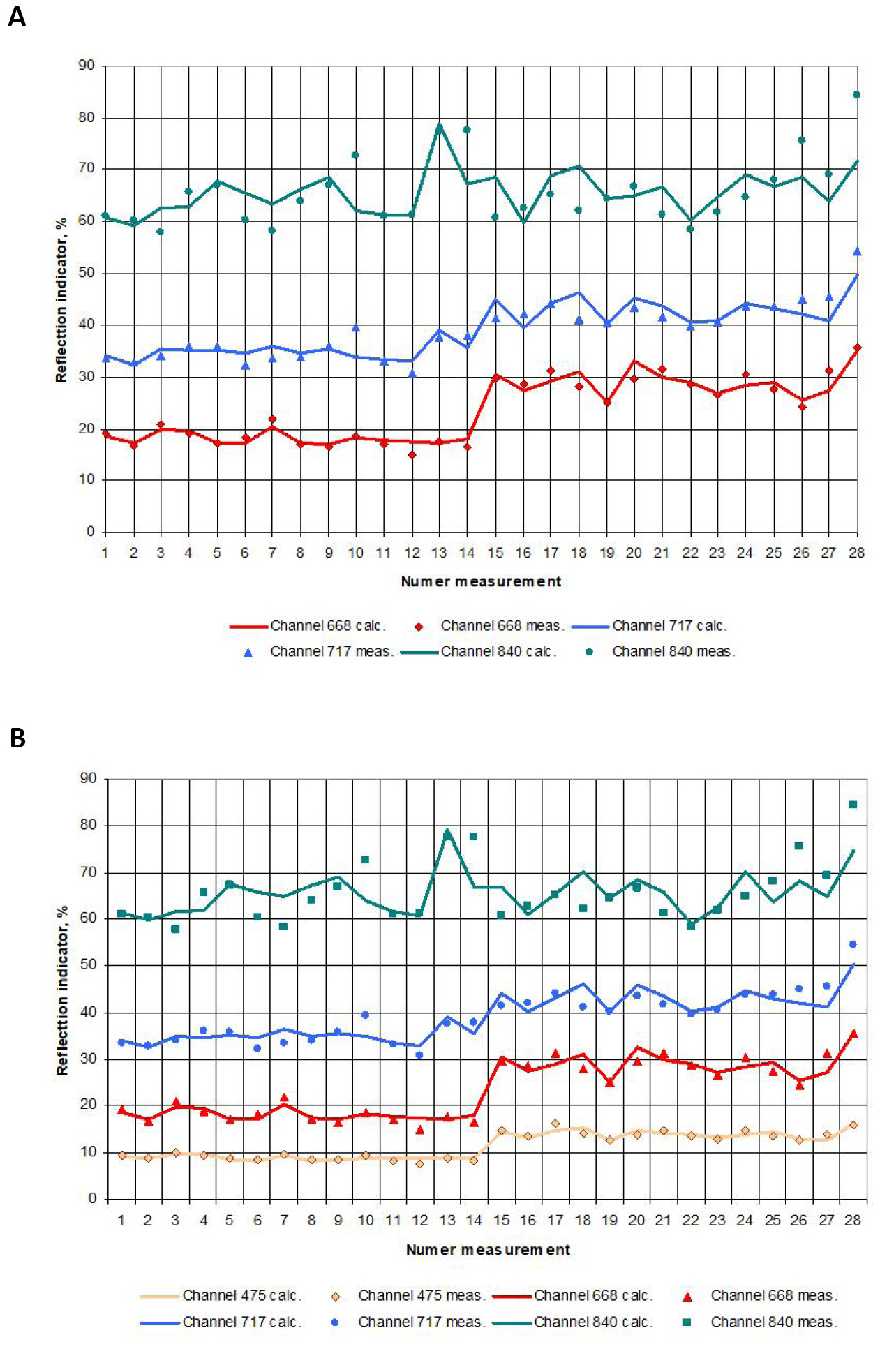
Figure 3. The process of identification of the ERS model. A: The process of identifying the ERS model for the agrocenosis in the time interval preceding the earing of spring wheat; B: The process of identification of the ERS model for the agrocenosis at the time interval between the phenophases of earing and full ripening of spring wheat.

 

On both graphs, the numbers of elementary plots (trial plots) were plotted along the horizontal axis. The experimental values of biomass indicators of agrocenoses were obtained, including crops of spring wheat and weeds. Reflection parameters (spectral brightness coefficients) were plotted along the vertical axis along the used spectral channels. For the period preceding the earing of spring wheat, these are green range (500-565nm); red (625-740nm) and near-IR (740-900nm). For the period between the phases of earing and full maturity, these are the green range (500-565nm), 1st red (625-700nm), 2nd red (700-750nm) and near-IR range (750-950nm). Thus, the geometric points on the graphs indicate the experimental values of the reflection parameters, and the solid lines reflect the calculated values of the reflection parameters obtained using models (6), (8).

 

As can be seen from the obtained identification results, both models show sufficient accuracy to solve the problem of estimating the parameters of agrocenoses using real remote sensing data. Modeling errors in models are maintained within ±10% tolerance. The model solutions uniformly cover the range of possible values of the reflection parameters and do not intersect with each other, which indicates the information of the spectral channels used.

 

Figure 4A shows the results of assessing the parameters of agrocenoses in the time interval preceding the phenophase of earing of spring wheat sowing.

 

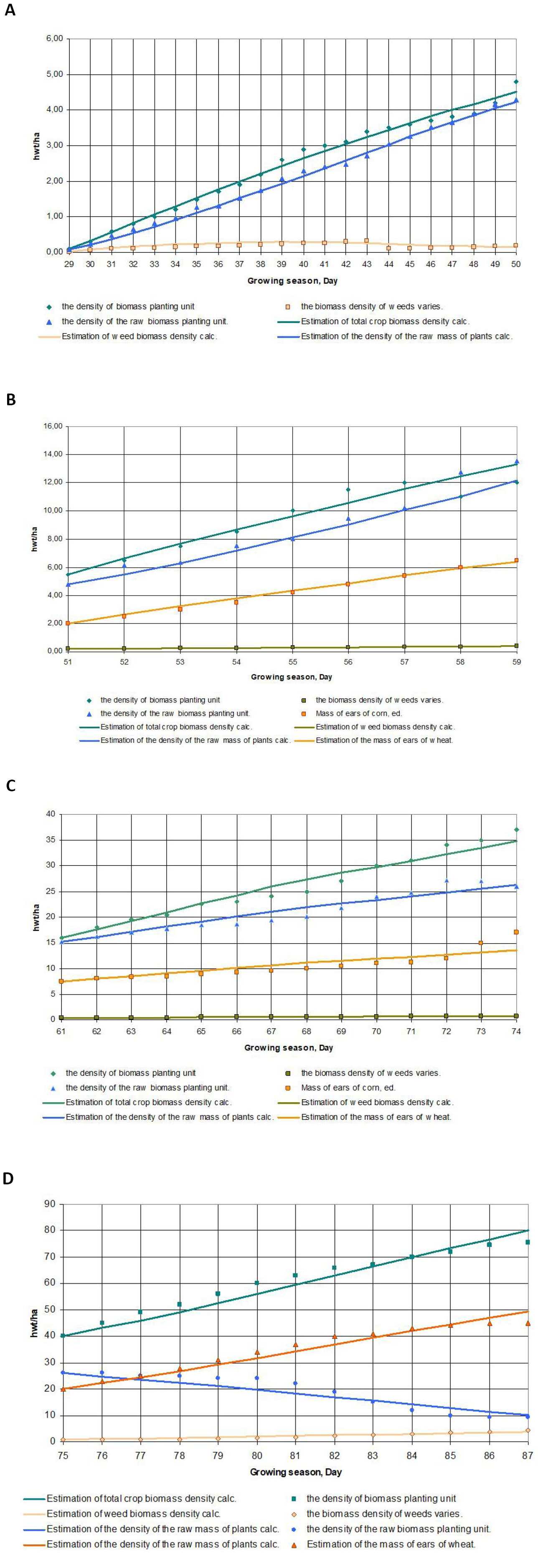
Figure 4. The process of evaluating the parameters of agrocenosis. A: The process of assessing the parameters of agrocenosis in the time interval preceding the phenophase of earing of spring wheat; B: The process of assessing the parameters of agrocenosis in the time interval between the phenophase of heading and flowering of spring wheat; C: The process of assessing the parameters of agrocenosis in the time interval between the phenophase of flowering and milky-wax ripeness of spring wheat; D: The process of evaluating the parameters of agrocenosis in the time interval between the phenophases of milky-wax ripeness and full ripening of spring wheat.

 

Along the horizontal axis, the time points in days of the considered growing season of the agrocenoses were plotted, and along the vertical axis, the geometric points represented the field-average experimental values of the parameters of the biomass of the agrocenoses, and the solid lines represent their estimates obtained from the remote sensing data. As can be seen from the graphs, the assessment process was stable, with its error within the tolerance of ±10%, which is adequate to address the issues in the management of the state of the agrocenoses.

 

An analysis of the experimental data on the parameters of the agrocenosis state and the results of the identification of the mathematical model (6) showed that with the same type of model, it has different parameter values at the intervals between phenophases, requiring the time interval from the beginning of heading to maturation into several interphase periods. The process of assessing the parameters of agrocenoses for these periods is shown in Figure 4B-4D.

 

As for the period preceding the phenophase of earing of spring wheat, the process of estimating the parameters of the agrocenoses biomass averaged over the field area was stable, and the estimation error remained a tolerance of ±10%.

 

Estimates of the field-averaged estimates of the biomass parameters of the main crop and weeds are available for the management decisions on fertilization rates and herbicide application rates over the entire field area. The differentiation of these technological operations required the assessment of the agrocenoses biomass parameters for all elementary areas. Moreover, the estimates for all elementary sections of the field were corrected using correctors (9). In contrast to the field-average parameter estimates, which are continuously constructed, correctors (9) were constructed only at the moments of the execution of the technological operation. Figure 5A-5C show the graphs for constructing spatial correctors for 20 test sites for selected points in time at different interphase periods of the growing season of sowing spring wheat.

 

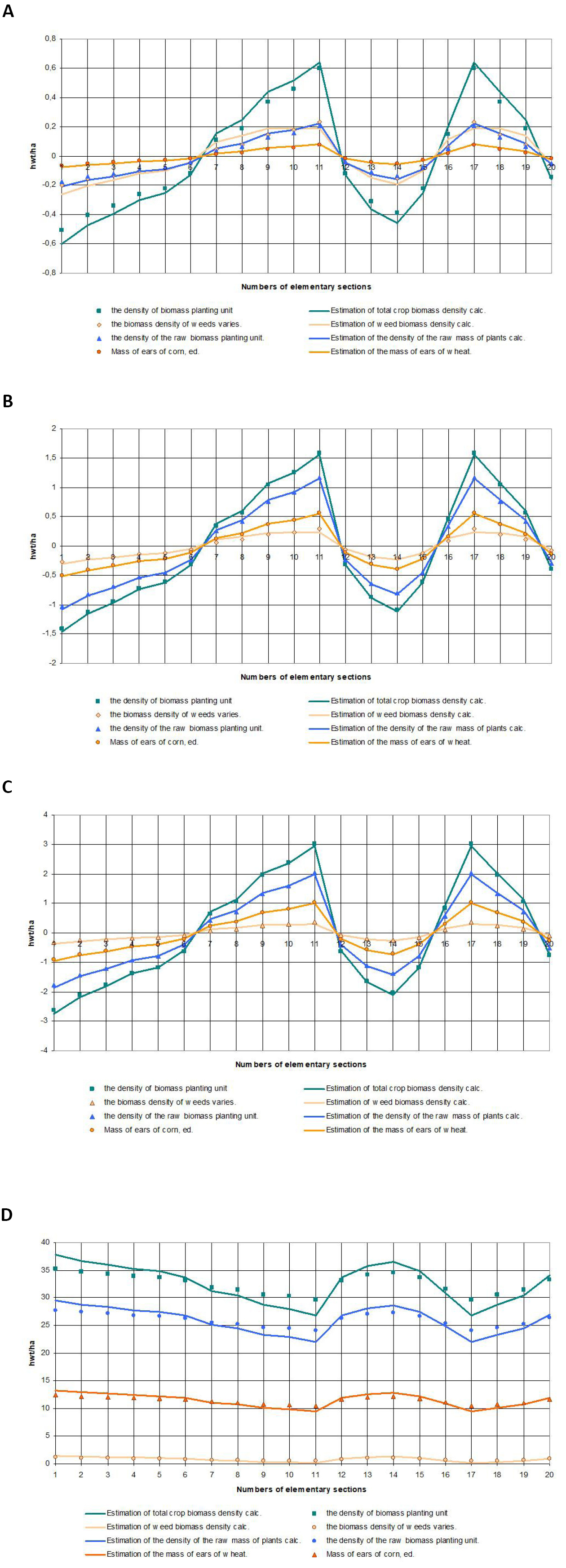
Figure 5. The process of identification of the spatial corrector. A: The process of identification of the spatial corrector for the 52nd growing season of sowing spring wheat; B: The process of identification of the spatial corrector for the 61st day of the growing season of sowing spring wheat; C: The process of identification of the spatial corrector for the 73rd growing season of sowing spring wheat; D: The process of spatial correction of biomass parameter estimates for the 73rd day of growing season of sowing spring wheat.

 

These results indicate a high similarity among these processes because the same elementary sections were used to construct the correctors. However, they significantly differed in the amplitudes of settings, which is associated with the processes of increasing biomass, leading to alterations in the parameters of spatial correctors. Figure 5D shows the graphs of the spatial correction of the parameters of the biomass of the agrocenoses for the 71st day of the growing season of spring wheat. Similarly, according to remote sensing data, estimates of the parameters of the agrocenoses were formed for the entire remaining area of the field for other points in time. These estimates are available to calculate local doses of mineral fertilizers and doses of weed treatments with herbicides.

 

4 DISCUSSION

To better understand the proposed methodology for assessing the parameters of agrocenoses, which includes the main crop (spring wheat) and weeds (specific species are not specified here), a general algorithm for the functioning of the information-measuring complex for assessment was presented in the current study (Figure 1).

 

Stage 0. Before beginning, all known parameters of mathematical models were introduced, which were obtained from the results of previous growing periods.

 

Stage 1. At the beginning of the tillering (germination) phase, samples of plants of the main crop and weeds were collected daily in real-time from trial plots or a field site. While sampling by stationary remote sensing means, the daily average parameters of the reflection of the agrocenoses on the test sites were formed. The obtained data were used to refine the parameters of mathematical models, which were carried out during the first 7 days.

 

Stage 2. From the 8th day, the mode of estimating the field-average biomass parameters according to the algorithm (10) was used for the entire growing season preceding the heading phenophase. If the technical operations of fertilizer application and herbicide treatment were performed during this period, mobile sensing tools were used to generate ERS data. In addition to the estimation algorithm (10), an algorithm for spatial correction of the agrocenoses state parameters was used accordingly (9).

 

Stage 3. From the onset of the earing phase, to a more complex morphological structure, and to the full maturity of the culture, the field-average parameters of the agrocenoses biomass were estimated according to the algorithm (9) and the stationary ERS tool, and during technological operations, the spatial correction of estimates was carried out according to the data of the mobile remote sensing device in accordance with formula (9).

 

An analysis of such studies, given in references[16-22], showed that the current models of crop yield losses from the impact of weeds, and models of weed competition with main crops have received the maximum development. According to such models, algorithms and decision support programs for weed control have been developed. However, the methodology for estimating the state parameters of agrocenoses containing the main crop and weeds based on remote sensing data has not yet been developed. Dynamic models of agrocenoses state parameters and remote sensing models, on the basis of which estimation algorithms are developed, are currently unavailable. The absence of such real-time evaluation tools significantly reduces the adequacy and reliability of decisions made on weed control.

 

5 CONCLUSION

The assessment of the parameters of the state of the biomass of agrocenoses, including the main crops and weeds, was carried out by combining ground-based measurements and ERS data. The problem of integration is related to the fact that ground-based measurements are point (local), and remote sensing data are distributed over the area of the field. To address this issue, a mathematical model of the dynamics of the parameters of the state of the agrocenoses biomass was used. This model has spatial coordinates and is a source of a priori information about the parameters of the agrocenoses biomass state with consideration of all influencing factors. To clarify this information based on remote sensing data, a mathematical model of the relationship between the estimated state parameters and remote sensing data was introduced. This allows the combination of the parameters and data into a single evaluation algorithm that forms estimates of the parameters of the agrocenoses biomass state with sufficient accuracy by coordinating the physical dimensions of the models. Furthermore, ground measurements, including stationary remote sensing devices, were performed on selected 15-30 test sites with a similar composition of agrocenoses, with an area of 10-20m2 and different doses of fertilizers, irrigation rates and varying degrees of weed infestation. Ground-based measurements were used to estimate the parameters of mathematical models, and remote sensing data from mobile remote sensing devices were used to form estimates of the biomass parameters of agrocenoses over the entire field area. To simplify the evaluation procedure, it was implemented in two stages. The first stage involved the formulation of the estimates of agrocenoses biomass parameters averaged over the area, and the second stage involved the correction of elementary plots using a linear spatial corrector. Therefore, the identification of the species composition of weeds and their share in the total biomass is of great significance. Moreover, the problem of model and evaluation algorithms establishment for other crops and agrocenoses is relevant.

 

Acknowledgements

Not applicable.

 

Conflicts of Interest

The author declared no conflict of interest.

 

Author Contribution

Mikhailenko IM solely contributed to this manuscript.

 

Abbreviation List

ERS, Earth remote sensing

UAV, Unmanned aerial vehicle

 

References

[1] Kriegler FJ, Malila WA, Nalepka RF et al. Preprocessing transformations and their effects on multispectral recognition: Proceedings of the Sixth International Symposium on Remote Sensing of Environment, Ann Arbor, USA, 13-16 October 1969. Ann Arbor, MI: University of Michigan; 1969.

[2] Rouse JW, Haas RH, Schell JA et al. Monitoring vegetation systems in the Great Plains with ERTS. In: Freden SC, Mercanti EP, Becker MA ed. Third ERTS Symposium, Scientific and Technical Information Office, National Aeronautics and Space Administration; Washington, USA, 1973; 309-317.

[3] Jordan CF. Derivation of leaf-area index from quality of light on the forest floor. Ecology, 1969; 50: 663-666. DOI: 10.2307/1936256

[4] Lillesand TM, Kiefer RW. Remote sensing and image interpretation, 2nd edition. John Wiley and Sons: USA, 1987.

[5] Crippen RE. Calculating the vegetation index faster. Remote Sens Environ, 1990; 34: 71-73. DOI: 10.1016/0034-4257(90)90085-Z

[6] Antonov VN, Sweet LA. Monitoring of the state of crops and forecasting the yield of spring wheat according to remote sensing data. Geom, 2009; 4: 50-53.

[7] Bartalev SA, Lupyan EA, Neishtadt IA et al. Classification of certain types of agricultural crops in the southern regions of Russia according to MODIS satellite data. Issledov Zem iz kosm, 2006; 3: 68-75.

[8] Lawrence RL, Ripple WJ. Comparisons among vegetation indices and bandwise regression in a highly disturbed, heterogeneous landscape: Mount St. Helens, Washington. Remote Sens Environ, 1998; 64: 91-102. DOI: 10.1016/S0034-4257(97)00171-5

[9] Ponzoni FJ, Borges da Silva C, Benfica dos Santos S et al. Local illumination influence on vegetation indices and plant area index (PAI) relationships. Rem Sens, 2014; 6: 6266-6282. DOI: 10.3390/rs6076266

[10] Sims DA, Gamon JA. Relationships between leaf pigment content and spectral reflectance across a wide range of species, leaf structures and developmental stages. Remote Sens Environ, 2002; 81: 337-354. DOI: 10.1016/S0034-4257(02)00010-X

[11] Mikhaylenko IM, Timoshin VN, Malygin VD. Decision-making on the date of fodder harvesting based on remote sensing data of the earth and mathematically tuned models. Decis Mak, 2018; 15: 169-182. DOI: 10.21046/2070-7401-2018-15-1-169-182

[12] Mikhailenko IM, Timoshin VN. Assessment of the chemical state of the soil medium according to remote sensing of the earth. Earth Space, 2018; 18: 125-134.

[13] Mikhailenko IM, Timoshin VN. Development of a methodology for assessing the parameters of the state of crops and soil environment for crops according to remote sensing of the Earth. IOP Conference Series: Earth and Environmental Science. IOP Publishing, 2020; 548: 052027. DOI: 10.1088/1755-1315/548/5/052027

[14] Mikhailenko IM, Timoshin VN, Weller VE. Estimation of the parameters of the state of the biomass of spring wheat crops [in Russian]. Bull Russ Agr Sci, 2021; 1: 2-6. DOI: 10.30850/vrsn/2021/1/4-8

[15] Kazakov IE. Methods for optimizing stochastic systems, Moscow, Russia, 1987.

[16] Bagavathiannan MV, Beckie HJ, Chantre GR et al. Simulation models on the ecology and management of arable weeds: structure, quantitative insights, and applications. Agron, 2020; 10: 1611. DOI: 10.3390/agronomy10101611

[17] Cousens R. An empirical model relating crop yield to weed and crop density and a statistical comparison with other models. J Agr Sci, 1985; 105: 513-521. DOI: 10.1017/S0021859600059396

[18] Christensen S. Crop weed competition and herbicide performance in cereal species and varieties. Weed Res, 1994; 34: 29-36. DOI: 10.1111/j.1365-3180.1994.tb01970.x

[19] Kropff MJ, Spitters CJT. A simple model of crop loss by weed competition from early observations on relative leaf area of the weeds. Weed Res, 1991; 3: 97-105. DOI: 10.1111/j.1365-3180.1991.tb01748.x

[20] Berti A, Bravin F, Zanin G. Application of decision-support software for postemergence weed control. Weed Sci, 2003; 51: 618-627. DOI: 10.1614/0043-1745(2003)051[0618:AODSFP]2.0.CO;2

[21] Neuho D, Schulz D, Köpke U. Potential of decision support systems for organic crop production: WECOF-DSS, a tool for weed control in winter wheat: In Proceedings of the International Scientific Conference on Organic Agriculture, Adelaide, Australia, 21-23 September 2005.

[22] Benjamin LR, Milne AE, Parsons DJ et al. Using stochastic dynamic programming to support weed management decisions over a rotation. Weed Res, 2009; 49: 207-216. DOI: 10.1111/j.1365-3180.2008.00678.x

 

Copyright © 2022 The Author(s). This open-access article is licensed under a Creative Commons Attribution 4.0 International License (https://creativecommons.org/licenses/by/4.0), which permits unrestricted use, sharing, adaptation, distribution, and reproduction in any medium, provided the original work is properly cited.