Analysis of the Interaction of Oceanic Cloudiness with the Upper Oceanic Stratum

 

Éric Zeltz1

 

1Independent Researcher, La Motte en Champsaur, Hautes-Alpes, France

 

*Correspondence to: Éric Zeltz, Independent Researcher, 5 route du Moulin, La Motte en Champsaur, Hautes-Alpes, 05500, France; Email: ericzeltz@wanadoo.fr

 

DOI: 10.53964/jia.2024004

 

Abstract

Objective: This paper addressed the relationship between two physical quantities of interest in climatology: the thermal energy present in the upper ocean stratum (UOS) and the oceanic cloudiness (OC), i.e., the one located above oceans.

 

Methods: The interplay between these physical quantities was pointed out by analyzing the time series of seasonal and diurnal anomalies of ocean's total cloud cover, and the anomalies of the thermal energy present in the UOS. We examined these time series to identify signals indicative of interactions between the UOS and OC. We then aimed to explain these interactions at a climatological level. Finally, for validation, we demonstrated that our explanations are consistent with a global climatological model that we developed.

 

Results: It was demonstrated that in both cases, the time series could be described as a Markov-1 alternating type, exhibiting similar structures. This led to the conclusion that the OC served as a natural thermostat in relation to the thermal energy contained in the UOS. By using a simple mathematical model previously introduced in a recent paper by the author (2023) to account for the thermal exchanges between the troposphere and the UOS, we confirmed that the OC acted as a natural thermostat for the thermal energy in the UOS. This "natural thermostat" effect, incorporated in the model, resulted in simulations projecting significantly less warming by 2095 compared to those from most existing global climate models (GCMs).

 

Conclusion: Methodologically, this paper confirmed the interest of using Markov chains to identify climatological interactions. The developed GCM, utilized for validating hypotheses explaining these interactions, proved simple and efficient for simulating key climatological parameters in the evolution of the global climate. On a strictly scientific level, the work's main contribution lies in providing a definitive answer about cloud cover feedback in global warming, establishing it as significantly negative.

 

Keywords: climate modeling, time series, Markov chains, ocean cloudiness, upper ocean stratum, natural thermostat

 

1 INTRODUCTION

The role of clouds and their interactions with climate-influencing factors, especially sea surface temperature (SST) and thermal energy in the upper ocean stratum (UOS), was not well understood[1-17]. A clear example of this situation is that of the recent historical evolution of the SST and the low cloud feedback over the Pacific region from the 1980s, which did not correspond to the response predicted by the global climate models (GCMs) taking into account the increase in CO2 that took place during this period[1-10]. Indeed, for the period between 1980 and 2014, Myers et al.[1] estimated that the difference between the cloud feedback arising from increasing abrupt-4x CO2 (i.e. impose an instantaneous quadrupling of the concentration of CO2 from the global annual mean 1850 value, then hold fixed) and the cloud feedback observed was of 0.78±0.21W·m-2·K-1 (90% Confidence Interval). Numerous hypotheses have been proposed to explain this significant distortion. Myers et al.[1] linked it to changes in SST independent of climate change and which are not taken into account by GCMs. Hartmann[2] believed that it corresponded to the appearance of the ozone hole in Antarctica from around 1980. Heede et al.[3] proposed the explanation that greenhouse gas-related warming is temporarily masked in the Pacific by aerosol effects. Kostov et al.[4] believed that the Southern Annular Mode (SAM) played an important role ignored by GCMs. For Rye et al.[5], it is the melting of the Antarctic ice sheets which is the driving force behind the unanticipated cooling. Seager et al.[6] attributed this distortion to a structural inability of GCMs to capture a correct response in the many regions sensitive to tropical Pacific Sea surface temperatures. For Seethala et al.[7] the changes observed in subtropical stratocumulus since the 1980s were attributed to natural variability, rather than a systematic response to climate change. Sherwood et al.[8] proposed an explanation for this distortion, citing the negative phases of the Pacific interdecadal oscillation and the SAM, as well as external forcings not captured by the models. Wanatabe et al.[9] believed that warming over this region of the Pacific was limited during this period from the 1980s onward by past trends in the equatorial Pacific Sea surface temperature gradient, which were not considered in the models. Finally, Wills et al.[10] believed that the distortion comes largely from systematic biases of the models, for example in the response to historical forcing, or in the taking into account of multi-decadal variability.

 

There were as many hypotheses as papers, with some overlap at times. This was expected, as with a single real-world climate system, robustly identifying the 'forced response' in observations is challenging.

 

This is why any improvement in the knowledge of the interactions between the UOS and the oceanic cloudiness (OC) can only increase the reliability of forecast climatology models[11-17]. Moreover, one of the major challenges listed by the World Climate Research Program consisted precisely in improving the understanding of the role of clouds in the climate[17].

 

This article examined relationships between the OC and the heat included in the UOS, in order to better understand the global mechanisms which govern their interaction.

 

Time series was analyzed concerning these two climatic entities with the aim of detecting possible “signals” of an interaction between them, by using a method introduced in Zeltz[18] for treating a similar climatological problem.

 

It turned out that they both presented the same probabilistic structure indicating a very precise interaction between the two entities, which led us to formulate the following hypothesis: the OC played the role of a natural thermostat for the UOS.

 

This explanation was validated with numerical simulations obtained by adapting the proposed model in Zeltz[18]. From 250 simulations by taking into account the natural thermostat effect of the OC, an increase between 1955 and 2095 in the SST of 0.47±1.6℃ (95% confidence), and an increase in that of the global atmospheric temperature of 0.40±1.2℃ (95% confidence) were estimated.

 

This was much lower than the projections obtained by the GCMs of national or international climatological institutes, in all the scenarios considered concerning Greenhouse Gas (GHGs).As for the progression over the same period of overall cloudiness, it would be 1.48%±1.4% (95% confidence).

 

All three projections were based on continuing GHGs in the atmosphere continued at the average rate observed over the historical period 1955-2023. This was incorporated into the model through the correlation with increased ocean stratification in the same period[18-20].

 

In addition to the previous projections, which were significantly lower than those appearing in the last IPCC report[21], our work made it possible to give a global explanation to phenomena like those reported at the beginning of this introduction and which, in our opinion, had until now been explained in ways that are as varied as they are unsatisfactory. With the simulations from our model, there is no longer this distortion described above with historical observations over the Pacific. They are in good coherence with the natural thermostat phenomenon of the OC on the UOS which is programmed in the model. The obtained result was that the oceanic nebulosity played a mitigation role in the temperature increasing of the SST due to GHGs in the atmosphere.

 

2 METHODS

2.1 Description of the Data Processing Method

To analyze the time series involved, we use a data processing method introduced and implemented recently[18,22] and of which here are the main steps:

(1) From the initial time series, derive a second one made up of “gaps”, i.e. the difference of a term of the initial series with the one which immediately precedes it.

(2) Then ensure that the derived series thus obtained can be modeled by what is called “white noise”[23], i.e.: without trend, neither for the expectation nor for the standard deviation, and having its own empirically calculated correlations almost zero and independent of their positions in time.

(3) This being verified, form a third series of 1s and 0s by associating each “gap” with the number 1 if it is positive, 0 otherwise.

(4) Then ensure that the point frequencies of 0 and 1 are both close to 0.5, which allows us to consider that the rises or falls of the quantitative character studied are equiprobable.

(5) This last observation, and the fact that the differences can be modeled by white noise, allows us to think that the series of 0 and 1 involved can be modeled by Markov series[23]. Given the relatively weak “climatic memory”[24-27] at play in the phenomena studied, this justifies that only three probabilistic situations will be considered: (a) Situation where each value of the series of 0 and 1 is independent of the previous one and where therefore the series of n elements is governed by a binomial law with parameters n and p=0.5 (“Markov-0 binomial” case). (b) Situation where each value in the series depends on the previous one in the sense that if the value of the previous one is 0(1), the next one has a greater probability of being 0(1) (“Markov-1 lengtheting " case). (c) Situation where each value in the series depends on the previous one in the sense that if the value of the previous one is 0(1), the next one has more probability of being 1(0) (“Markov-1 alternating” case).

 

In order to make a decision between these three possibilities, it remains to compare the average lengths of the “chains of rises” of successive 1s and those of the “chains of descents” of successive 0s in relation to the theoretical average length which for a binomial law with parameters n=100 and p=0.5 is 1.98. The criteria defined under this situation will be used in Zeltz[18,22]: If the average length of the ascending chains and the descending chains is less than 1.80, the initial series is of the “Markov-1 alternating” type; between 1.80 and 2.10, of “Markov-0 binomial” type; greater than 2.10, of the “Markov-1 lengthening” type. In all cases, an estimate of the probability assuming that the series of 0 and 1 is modelled by a Bn binomial distribution.

 

Finally, if for the two series studied the previous process comes to an end, which is not obligatory, it will be enough to compare the signals obtained to check whether there is a highly probable interaction or not between the two entities studied. If the answer is positive, all that will remain is to specify the underlying climatological mechanism.

 

2.2 Presentation of Data Used for the OC

Although great efforts have been made in recent years in this area, obtaining reliable data on cloudiness remains problematic[28-30]. A recent article[31] takes stock of what several different satellite sources have obtained on this and Figure 1 presents the graphs of the global cloud cover anomalies they give for the period 1983-2022. The means used by the institutes that produced these data are at the cutting edge of current technologies: NASA's Aftermoon-Train (A-Train) sensors with medium-resolution imaging spectroradiometer (MODIS) on board the Aqua satellite, cloud-aerosol lidar with orthogonal polarization (CALIOP), Pathfinder infrared satellite observations (CALIPSO), cloud profiling radar on board satellites (CPR), etc.

 

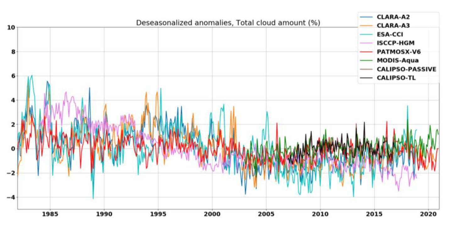
Figure 1. De-seasonalized anomalies of global mean total cloud amount (%) derived from four cloud CDRs as well as from MODIS-Aqua and CALIPSO. The trends in CLARA-A3, PATMOS-x, ESA-CCI, ISCCP-HGM are −0.76%, −0.28%, −0.82% and −1.47% per decade, respectively. All trends are statistically significant based on Mann Kendall test. Source: Devasthale and Karlsonn[31].

 

However, large disparities between the different results obtained were seen. The optimism expressed a few years ago (see for example Bony et al.[32]) for the rapid achievement of convergent and reliable results is therefore not yet fully validated by the facts.

 

In addition, all these data concern the cloudiness present over the entire Earth, and not just the OC. However, it seemed essential to us that the database would be used met these two criteria: (1) Focus only on the cloud cover above the oceans, so that terrestrial influences do not confuse the analysis of the interactions of the OC with the UOS. (2) Cover a sufficiently long and at the same time recent enough period to verify whether the global warming proven since the 1970s modifies the mechanism of interactions between the two entities.

 

A database respecting these two criteria, to our knowledge there are no others, is from Eastman et al.[33] which represented by the graph in Figure 2. These are the quarterly average diurnal OC anomalies for the period 1954-2008 obtained from meteorological reports taken on board ships and updated to Organization standards. World Weather Service to form an “Extended Edited Cloud Reports Archive” (EECRA)[34] which corresponds to the criteria specified above and led us to favor it. Some additional details about it:

- Its authors did not use the nighttime data available to them because they were not always numerous enough to obtain sufficiently reliable results.

- On the other hand, in the 10×10 grid boxes where there were a sufficient number of them, they were able to verify their good correlation with the diurnal data.

- Likewise, they found that the results were very similar to those purely diurnal using the day/night averages where those of the nights are confused with those of the days in the cells where the number of nighttime measurements is insufficient to obtain 'a reliable.

- Despite certain limitations inherent to the technique used, for example the fact that medium and high-altitude clouds are often masked by lower clouds, the authors estimated the uncertainties in these data to be less than 5%.

 

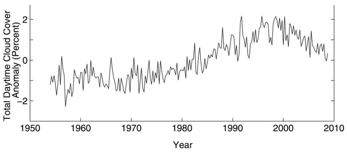
Figure 2. Global Time Series of Seasonal and Diurnal Anomalies of Total Cloud Cover Calculated for Ocean Areas Over the Period 1954-2008.

 

In Figure 2, no attempt has been made to eliminate parasitic variations over the ocean. Over the ocean, seasonal anomalies for each season were calculated for each 10×10 grid square. The seasonal anomalies in each box were then averaged to form overall seasonal anomalies, weighted by the relative area of the box and the ocean fraction. Source: Eastman et al[33].

 

2.3 Impact of Data Uncertainties on the Signals Obtained

Therefore, a time series of 220 data points were given which we will process as we described in paragraph 2.1. Among the advantages of this method already well highlighted in Zeltz[18,22], one will play a crucial role in relation to the large uncertainties in the initial data: even if these are provided with a notable uncertainty like this is the case with the OC data, this uncertainty disappears to a large extent concerning the signals 0 or 1 attached to the descents or rises from one quarter to the next. As for the nature of the signal, the probability that it will change given the uncertainty in the initial data is tiny. Unless it is “border”, that is to say the average length of its chains is very close to 1.80 or 2.10.

 

Indeed, we verified that even if the uncertainty in the initial data values was 20% (±10%), the signal 0 or 1 will remain unchanged with a confidence threshold greater than 94%. If the uncertainty in the data values was 10% (±5%), the signal 0 or 1 will remain unchanged with a confidence threshold greater than 96%. If the uncertainty in the data values was 5% (±2.5%), the signal 0 or 1 will remain unchanged with a confidence threshold of 98.3%. However, the uncertainty in the OC data used is evaluated by Eastman et al.[33] less than 5%. So, unless the average chain lengths are very close to one of the two boundary values 1.80 or 2.10, the type of signal obtained is very robust.

 

2.4 Signal Attached to OC Data

After verified the series derived from its deviations could be modeled by white noise (steps 1 and 2 of the method described in paragraph 2.1), then successfully verified the quasi-probability of the responses 1 and 0 (steps 3 and 4), we can draw up the table allowing us to identify the signals carried by the OC data studied (Table 1).

 

Table 1. Average Frequencies by Length of Chains of OC Anomalies for Series of 100 Quarters

Notes: Last line: frequencies and theoretical average length of the chains (rise or fall) for the binomial law B100 with parameters n=100 and P=0.5.

 

We noted that over the two periods of 100 consecutive quarters observed, the signals were clearly of the Markov-1 alternating type. The reality of this behavior of forced alternation is therefore very probable. On the contrary, in the context of governance by the B100 binomial distribution, the probability of having such small values for average lengths were very low (about one chance in two hundred). This was confirmed over the total period of 220 quarters between 1954 and 2009 as shown in Table 2.

 

Table 2. Results Between 1954 and 2009

Notes: Same types of results as for Table 1 but for the entire period 1954-2009 studied, i.e. for 220 consecutive quarters.

 

Furthermore, we did not note any particular change between before and after proven warming (1970).

 

2.5 Robustness of The Signal Attached to Cloudiness Anomalies

To verify that the signal obtained does not come from any bias coming from the data themselves collected at sea level, we tested the type of signals obtained from four databases from satellite observations of the Daytime cloudiness between 60°S latitude and 60°N latitude. The first three are studied by Norris and Evan[35] and the last by Rossow et al[36]. Here are the precise origins of this data and the periods concerned:

-The first concerns the period 1984-2009 and comes from the ISCCP: https://eosweb.larc.nasa.gov/project/isccp/isccp_table

-The second, again for the period 1984-2009, comes from PATMOS-x: http://cimss.ssec.wisc.edu/patmosx/data

-The third for the period 2002-2015 by Aqua MODIS. http://ladsweb.nascom.nasa.gov/data/search.html

-The fourth for the period 1984-2018 by ISCCP-H: https://www.ncei.noaa.gov/access/metadata/landing-page/bin/iso?id=gov.noaa.ncdc:C00956

 

We treated these data in the same way as those from Eastman et al.[33] with whom we obtained Tables 1 and 2. Table 3 presents the results achieved:

 

Table 3. Average Frequencies by Length of Chains of Diurnal Cloudiness Anomalies for Series of Quarters

Notes: Last line: frequencies and theoretical average length of the chains (rise or fall) for the binomial law B100 with parameters n=100 and P=0.5.

 

We found in all cases the type of signal encountered for the OC: for the four data series considered, the diurnal cloudiness anomalies of the portion of the Earth between 60°S latitude and 60°N latitude have “Markov-1 alternating” type well pronounced. Therefore, the change in technology, the different periods considered, the fact that terrestrial parts and not just oceanic parts are considered, finally the restriction of the study to the part of the planet between 60°N latitude and 60°S latitude, all this does not affect the quality of the signal, which therefore appears to be a very robust characteristic of cloudiness. This means that the interaction between the OC and the heat of the UOS has a strong enough impact that it is visible throughout the nebulosity of the terrestrial globe.

 

2.6 Signal Attached to UOS Heat Data

For the heat data (thermal energy) present in the UOS, we used a database from NOAA and already used by a previous research[18]. The link to download it is: https://www.climate.gov/media/13603. It only begins with the year 1955 and therefore covers 216 quarters from 1955 to 2009 in common with the previous OC database.

 

As Table 4 clearly indicates, we arrive at the same observation as for the OC, namely a clearly Markov-1 alternating type signal for the two chains of 100 quarters considered:

 

Table 4. Average Frequencies of Appearance by Length of UOS Thermal Variation Anomalies Present for Series of 100 Quarters

Notes: Last line: frequencies and theoretical average length of the chains (rise or fall) for thebinomial law B100 with parameters n=100 and P=0.5.

 

Table 5 shows that the same is true for the complete chain of 216 quarters of the period 1955-2009.

 

Table 5. Same Types of Results as for Table 3 but for the Entire Period 1955-2009 Studied

Notes: for 216 consecutive quarters.

 

From the same ocean heat anomaly data source, this Markov-1 alternating type character had already been identified by Zeltz[18] over a longer period (1955-2022) for the 3 chains of 90 consecutive quarters concerned. Thus, the reality of this character for the thermal energy of the UOS is, as for the OC, very highly probable.

 

On the other hand, the probability of having such small average lengths of the three chains would be very low if they were governed by the B90 binomial distribution: about one chance in five hundred.

 

2.7 Comparative Trends in the Two Datasets Studied

Figure 3 presents the variation graphs for the common period 1955-2009 of OC anomalies(%) and UOS heat (1u.=5×1022J).

 

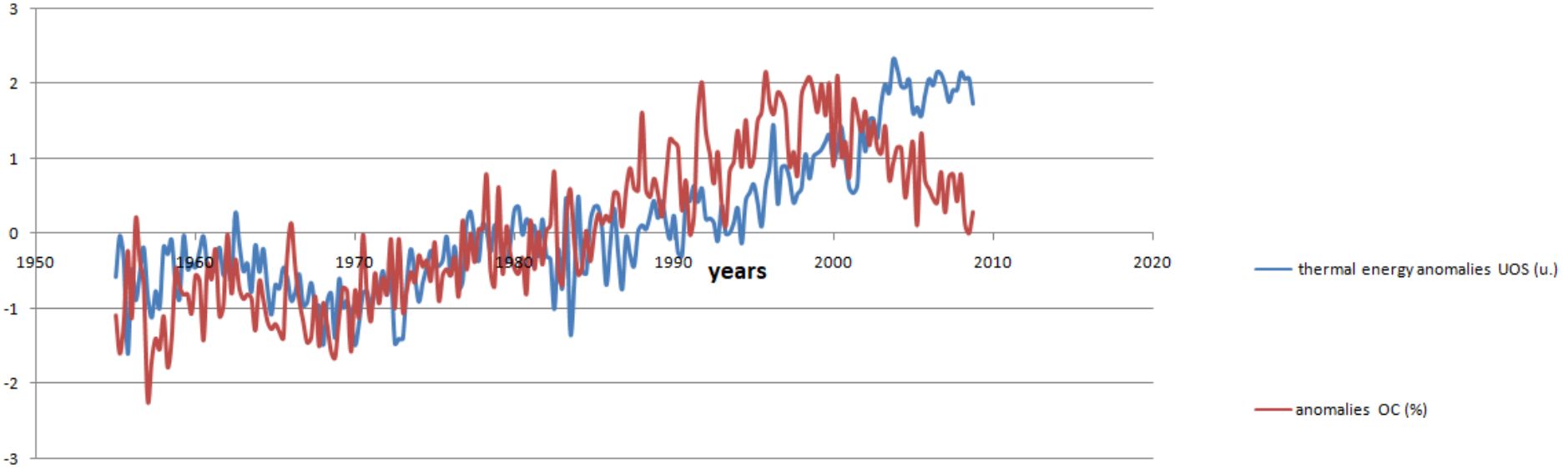
Figure 3. Variations in OC anomalies in % (red curve) and heat anomalies in UOS (blue curve. 1u.=5×1022J) for the common study period 1955-2009.

 

The correlation between the two series is significant (0.65). Overall, the two curves show fairly clear growth, although for OC there was a remarkable decline in the last decade of the study. (Remarks: The decline over this same period is also observable in most of the curves in Figure 1. Then, most of them show an upturn until the present day.)

 

3 RESULTS AND DISCUSSION

3.1 Climatological Interpretations

As observed, the two “signals” on the quarterly data studied in the previous paragraph are frankly of the Markov-1 alternating type and they are also significantly correlated. It therefore seems natural to us to explain this by an interaction between the OC and the thermal energy of the UOS, the mechanism of which would be as following explanations.

 

During a quarter the UOS warms up, this causes additional evaporation which has the consequence of increasing low and medium cloudiness, either in surface area or in opacity power by increasing their density, which in both cases increases their cooling power. So when the production of this cloudiness develops following this warming, this new or more opaque cloudiness contributes to cooling what is under it, therefore the UOS, whose heat ends up starting to decrease with a certain delay. But then the production of cloudiness also begins to decrease since there is less evaporation, which in turn leads to further warming of the UOS, since it is better exposed to solar radiation. And so on. In our opinion, we are therefore dealing with an interaction that can be compared to a two-stroke engine whose pistons would be the heat of the UOS and the OC. As for the three-month cycles for the heat present in the UOS, they come from another interaction, the one that was highlighted by Zeltz[18] with the same “signal” techniques between the heat of the UOS and global average atmospheric temperature. Cycles which had been explained in particular by the cooling of the water which undergoes evaporation, but which the present study shows that they are undoubtedly further amplified by the reciprocal influence between the UOS and the OC.

 

According to this hypothesis, the clouds of the OC would therefore have the damping effect of a natural thermostat: when the heat of the UOS increases, they tend to reduce it following their increased development; when on the contrary it decreases, the OC regresses and therefore filters less solar radiation which therefore reaches the surface of the UOS more easily, increasing its heat.

 

3.2 Discussion

This hypothesis of the role of natural thermostat played by cloudiness has already been formulated in the climatological literature. In particular to explain why in tropical zones the impact of global warming is not as intense as in other regions of the globe (Miller's “thermostat” hypothesis[37] or that of Pierrehumbert[38]).

 

And our explanation which goes in the direction of a negative feedback of the role of clouds in current global warming is largely confirmed by certain more recent articles[39-42]. For example, according to Ceppi et al.[41], “A robust feature of global warming model experiments is a negative shortwave cloud feedback in the middle to high latitudes, driven by an optical thickening of the clouds associated with liquid water path (LWP) increases.” Or again for Ceppi et al.[42], “Using historical CMIP5 model data and satellite retrievals of cloud properties, we have shown that as the atmosphere warms, cloud liquid water (and hence optical depth) consistently increase in middle to high latitudes (poleward of ∼45°) in the Southern Hemisphere, with an additional weak cloud amount response to warming.” This is consistent with our hypothesis.

 

On the other hand, this seems contradictory with other recent theories and models which predict a drop in low cloudiness following the warming of the ocean surface temperature[43-46]. The main explanation put forward is that warming would have the effect of increasing the flow of latent heat at the surface, which would reinforce vertical mixing by convection in the lower troposphere and dry out the lower layers. But for example, Rieck et al.[43] remain very cautious in their conclusions and do not want to draw definitive conclusions on the fate of the lower layer following global warming. Because according to these authors, “the ultimate response of shallow convection in the trade winds may depend on subtle compromises between competing effects.”

 

Our explanation did not take into account many other phenomena which add up and enormously complicate the analysis of the evolution of the heat of the UOS and the OC. Indeed, just for the latter: evolution of atmospheric circulation, physics of clouds with for example very different effects depending on their type and altitude, stability or not of the troposphere, transparency or opacity of clouds, vertical movements of the humid air, presence or absence of aerosols, seasonal cycles, etc[47-50]. But the fact remains that the signals exhibited in the series studied are real and well marked: they certainly reflect an interaction that must be made explicit, which is what we therefore tried to do.

 

That said, the current research trend suggests that cloud feedback amplifies global warming[51-54] rather than moderating it. But the estimates of this feedback remain very imprecise: in 2013 and according Boucher et al.[51], between -0.09 and +0.99 W⋅m-2⋅K-1 at the 90% confidence threshold. However, these estimates are obtained by using all available data sources: theory, modeling, and Earth observations. The fact remains that despite all these efforts, a tight constraint on this feedback remains elusive. As stated in an article by Ceppi and Nowack[54], “theory cannot provide accurate projections, global climate models are unable to explicitly represent small-scale cloud processes, and limitations in computing power do not allow high-resolution models to perform experiments on the climate change” at the level of the entire planet. To try to overcome this, the latter authors developed ina statistical learning method that is said to “significantly improve on previous estimates and does not require high-resolution simulations or observations.”[54] But the range that they obtain at the 90% confidence threshold in their article dated 2021 still remains very wide: between +0.08 et +0.78W⋅m-2⋅K-1. Far from completely banning negative feedback.

 

3.3 Modeling of the Ocean/Atmosphere/Cloudiness Coupling

The Z.2 model which will be used to validate our hypothesis on the negative feedback of cloudiness, and to obtain simulations consistent with our explanations, is built from the Z.1 model developed by Zeltz[18]. Of the 17 lines of the tables on which the Z.1 model is based, only line 6 concerning the atmospheric albedo an has been modified. In model Z.1, it was written as in Table 6:

 

Table 6. Line 6 of Model Z.1

Line Number	Equation	Purpose	Illustration
6	an=an-1	Evolution of the atmospheric albedo.

 

In model Z.2, it splits into the following two sublines 6a and 6b(Table 7):

 

Table 7. Lines 6a and 6b of Model Z.2

 

The equality cln+1=cln+β(θn+1-θn) of 6a reflects the relationship between the OC and the heat present in the UOS explained in section 3.1 and updated in paragraph 2 by the presence of the signals of “Markov-1 alternating” type on each of their data series. The estimation of the constant β was made by “calibration” with the data of the OC anomalies presented in section 2.2 and coming from the EECRA[34].

 

Line 6b makes it possible to evaluate the atmospheric albedo. It is assimilated to that generated by the OC because that coming from the ocean surface is negligible compared to that of the clouds[55,56]. Furthermore, according to Wen et al.[56], the reflectance of clouds located above the oceans, and therefore their albedo, depends linearly on their coverage [Cf. formula (5a)[56]]. This justifies the relation an=γ×cln of line 6b. Konsta[57] allowed us to obtain the provided estimate of the constant γ [See 4.2.1(a)[57]].

 

The following Table 8 lists the relationships used by the Z.2 model. For the other 16 lines of the table common with those of model Z.1 (lines 1 to 5 and 7 to 17), the notations introduced and the relationships used are briefly explained. More details are given in paragraph3.3 of Zeltz[18].

 

Table 8. Summary of the Relationships Founding the Model Z.2 and Complementary Relationships

 

3.4 Simulations

Figure 4 compares simulations obtained using the two models for the period 1955-2095.

 

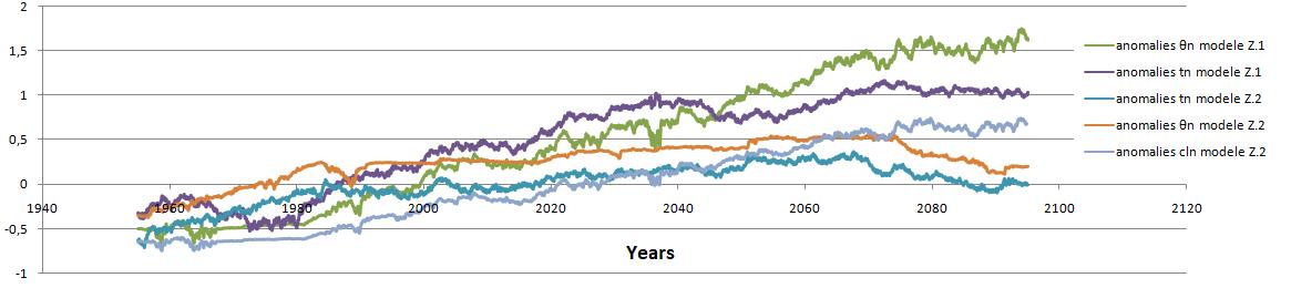
Figure 4. Graphs concerning simulations made on θn, tn and cln for the period 1955-2095. Simulations of θn and tn anomalies (℃) obtained with the Z.1 model. (respectively green and purple curve). Simulations of θn and tn anomalies (℃) obtained with the Z.2 model (respectively orange curve and blue curve). Simulations of cln anomalies (%) obtained with the Z.2 model (light blue curve).

 

The feedback predicted by our hypothesis is clear in these graphs since in 2095, the end of the simulation, the temperatures provided by the Z.2 model are lower than those provided by the Z.1 model, by about 1.5℃ for θn and 1℃ for tn. Table 9 shows the theoretical figures in terms of mathematical expectation that allow us to compare the two models and to measure the theoretical feedback predicted by the Z.2 model for the period 1955-2095.

 

Table 9. Comparison of the Heoretical Progressions Predicted by The Two Models

 

The expected negative feedback is therefore well taken into account by the Z.2 model and is not at all negligible. In Annex, we present two other simulations provided by our Z.2 model.

 

3.5 Z.2 Model CI Results

From 250 simulations provided by the Z.2 model, we constituted three samples of 250 values as follows:

(1) First S1 sample consisting of the 250 cl1680-cl1 values associated with each of the 250 cln simulations over the period 1955-2095.

(2)Second S2 sample consisting of the 250 t1680-t1 values associated with each of the 250 tn simulations over the period 1955-2095.

(3)Third S3 sample consisting of the 250 θ1680-θ1 values associated with each of the 250 θn simulations over the period 1955-2095.

 

After being able to positively test the normality of these three samples, we determined the 95% confidence intervals for the progressions over the entire period 1955-2095 of cln, tn and θn provided by our Z.2 model.

 

To do this, we took as parameters μ and σ normal distributions at play:

(1) For the μ means, the mathematical expectations already indicated in Table 7 (the point averages of S1, S2 and S3 being very close to them, as we have checked).

(2) For standard deviations σ, estimates obtained from the point standard deviations of S1, S2 and S3.

 

Table 10. Normal Distribution Parameters Involved and 95% Confidence Intervals Obtained from Samples S1, S2 and S3

Progress Over the Period 1955-2095	μ	σ	[μ-2σ; μ+2σ]
cl1680- cl1	+0.35%	0.29%	[0.06%; 0.64%]
t1680- t1	+0.49℃	0.16℃	[0.33℃; 0.65℃]
θ1680- θ1	+0.43℃	0.15℃	[0.28℃; 0.58℃]

 

3.6 Correlations Between S1, S2 and S3 Samples

According to the hypotheses taken into account by model Z.2, we should expect significantly positive correlations between S1 and S2, between S1 and S3 and finally between S2 and S3. This is what is observed:

 

Table 11. Correlations Between Samples S1, S2 and S3

 

Additional remarks on the models and simulations obtained:

(1) The simulations shown in Figure 4 use the same values for all constants common to the Z.1 and Z.2 models for both models of tn and θn, and the same for the random coefficients used in both models to account for natural variability.

(2) The same applies to the simulations shown in Supplementary Figures 1 and 2.

(3) As shown in Figure 1, the increase in OC predicted by the Z.2 model is not contradicted by most observations over the past decade.

(4) Simulations are very easily and quickly obtained using a conventional spreadsheet and a simple microcomputer. For example, we were able to generate the 250 simulations in less than an hour that allowed us to reach the confidence intervals for the total changes cl1680-cl1, t1680-t1 and θ1680-θ1 of three variables simulated by the Z.2 model over the period 1955-2095.

(5) The author will send a copy of the Z.1 and Z.2 program free of charge by e-mail for any request that he or she deems justified.

 

4 CONCLUSION

The initial aim of this work was to study and clarify the interactions between the OC and the thermal energy contained in the UOS. The OC has the role of a natural thermostat vis-à-vis the UOS and has therefore already reduced and will further reduce the magnitude of global warming, which is probably largely anthropogenic and which has been observed since the 1970s.

 

For the 140-year period of the study (1955-2095), the model that was developed during this work and which is the development of a model introduced in Zeltz[18], estimates the action of this negative feedback on the temperature of the UOS at more than 2℃ and at more than 1℃ that on the global average atmospheric temperature. This global model is based on the energy equilibria and exchanges between the UOS, the troposphere, the stratosphere and solar heat. The exchanges between the heat of the atmosphere and that of the UOS had already been specified in Zeltz[18], using a method using "signals" revealing the processes at play and which appeared on the time series studied. This is the same technique that was used here and revealed the natural thermostat role that the OC played on the UOS. The consideration of everything else that influences the Earth's climate (winds, ocean currents, upward and downward convection, influences of land and vegetation, etc.) is taken into account in a very rudimentary but real way, thanks to a concept introduced of “dynamic heat capacity”[18]. It is obvious that this work, with the very modest model that is presented and used, did not claim to replace the monumental one carried out by the major International Climatological Institutes, in particular with the GCMs that they develop and use with the help of very powerful computers.

 

However, In our view, this research conclusively resolves the question of cloudiness feedback (particularly oceanic) in relation to global warming, showing it to be negative and significantly impactful. Moreover, it offers global insights into phenomena not well understood until now. For instance, as we pointed out in the Introduction, the significant distortion between historical data and GCM simulations which concern the SST evolution in the Pacific. For the simulations obtained by the Z.2 model which integrates this negative feedback, there is no longer this.

 

And so, therefore, GCMs, which were much more elaborate and complex than ours, should take it into account in order to arrive at more realistic and less imprecise results than they still are today, despite all the work and technology involved.

 

We will conclude by specifying two perspectives on this work which seem interesting to us: (1) In order to refine our Z.2 model, study the interaction of ocean stratification on global warming. (2) Explore the following hypothesis: The low interannual variability of global cloud cover[58,59], linked according to these authors to an equally low interannual variability of the Earth's albedo, perhaps comes, at least in part of the damping effect that the OC played on the heat of the UOS.

 

Acknowledgements

I sincerely acknowledge Jean Poitou, Jérôme Pousin and Salaheddine Skali-Lami for their proofreading of the manuscript and their valuable advice.

 

Conflicts of Interest

The author declared that there is no conflict of interest regarding the publication of this article. No potential conflict of interest has been reported by the author.

 

Author Contribution

The author participated in the drafting and writing of the manuscript. The author contributed to the manuscript and approved the final version.

 

Abbreviation List

A-Train, Aftermoon-train

CALIOP, Cloud-aerosol lidar with orthogonal polarization

EECRA, Extended edited cloud reports archive

GCM, Global climate model

GHG, Greenhouse gas

LWP, Liquid water path

MODIS, Medium-resolution imaging spectroradiomete

OC, Oceanic cloudiness

SAM, Southern annular mode

SST, Sea surface temperature

UOS, Upper oceanic stratum

 

References

[1] Myers TA, Zelinka MD, Klein SA. Observational constraints on the cloud feedback pattern effect. J Climate, 2014; 36: 6533-6545.[DOI]

[2] Hartmann DL. The Antarctic ozone hole and the pattern effect on climate sensitivity. P Natl Acad Sci USA, 2022; 119: e2207889119.[DOI]

[3] Heede UK, Fedorov AV. Eastern equatorial Pacific warming delayed by aerosols and thermostat response to CO2 increase. Nat Clim Change, 2021; 11: 696-703. [DOI]

[4] Kostov Y, Ferreira D, Armour KC et al. Contributions of greenhouse gas forcing and the Southern Annular Mode to historical Southern Ocean surface temperature trends. Geophys Res Lett, 2018; 45: 1086-1097.[DOI]

[5] Rye CD, Marshall J, Kelley M et al. Antarctic glacial melt as a driver of recent Southern Ocean climate trends. Geophys Res Lett, 2020; 47: e2019GL086892.[DOI]

[6] Seager R, Cane M, Henderson N et al. Strengthening tropical Pacific zonal sea surface temperature gradient consistent with rising greenhouse gases. Nat Clim Change, 2019; 9: 517-522.[DOI]

[7] Seethala C, Norris JR, Myers TA. How has subtropical stratocumulus and associated meteorology changed since the 1980s? J Climate, 2015; 28: 8396-8410.[DOI]

[8] Sherwood SC, Webb MJ, Annan JD et al. An assessment of Earth’s climate sensitivity using multiple lines of evidence. Rev Geophys, 2020; 58: e2019RG000678.[DOI]

[9] Watanabe M, Dufresne JL, Kosaka Y et al. Enhanced warming constrained by past trends in equatorial Pacific sea surface temperature gradient. Nat Clim Change, 2021; 11: 33-37.[DOI]

[10] Wills RCJ, Dong Y, Proistosecu C et al. Systematic climate model biases in the large-scale patterns of recent sea-surface temperature and sea-level pressure change. Geophys Res Lett, 2022; 49: e2022GL100011.[DOI]

[11] Bony S. Dufresne JL. Marine boundary layer clouds at the heart of tropical cloud feedback uncertainties in climate models. Geophys Res Lett, 2005; 32:L20806.[DOI]

[12] Nam C, Bony S, Dufresne JL et al. The ‘too few, too bright’ tropical low-cloud problem in CMIP5 models, Geophys Res Lett, 2012; 39:L21801.[DOI]

[13] Stephens GL. Cloud feedbacks in the climate system: A critical review. J Climate, 2005; 18: 237-273.[DOI]

[14] Tokinaga H, Tanimoto Y, Xie S et al. Ocean frontal effects on the vertical development of clouds over the Western North Pacific: In Situ and satellite observations, J Climate, 2009; 22: 4241-4260.[DOI]

[15] Schiro KA, Su H, Ahmed F et al. Model spread in tropical low cloud feedback tied to overturning circulation response to warming. Nat Commun. 2022; 13: 7119.[DOI]

[16] Fueglistaler S. Observational evidence for two modes of coupling between sea surface temperatures, tropospheric temperature profile, and shortwave cloud radiative effect in the tropics. Geophys Res Lett, 2019; 46: 9890-9898.[DOI]

[17] WCRP Grand Challenge on Clouds, Circulation and Climate Sensitivity. Accessed 2024. Available at:[Web]

[18] Zeltz É. Origins of "Natural Climatic Nervousness" and its current accentuation. J Mod Green Energy, 2023; 2: 8.[DOI]

[19] Li G, Cheng L, Zhu J et al. Increasing ocean stratification over the past half-century. Nat Clim Change, 2020; 10: 1116-1123.[DOI]

[20] Sallée JB, Pellichero V, Akhoudas C et al. Summertime increases in upper-ocean stratification and mixed-layer depth. Nature, 2021; 591: 592-598.[DOI]

[21] IPCC. Synthesis Report of the Sixth Assessment Report. Accessed 2024. Available at:[Web]

[22] Zeltz É. (2021), Analyse et interprétation climatologique de l'évolution des températures moyennes mondiales depuis 1880. Physio-Geo, 2021; 16: 49-70.[DOI]

[23] Hamilton JD. Time Series Analysis. Princeton University Press: Princeton, USA, 1994; 799.

[24] Shukla J. Dynamical predictability of monthly means. J Atmos Sci, 1981; 38: 2547-2572.[DOI]

[25] Buizza R, Leutbecher M. The forecast skill horizon. Q J Roy Meteor Soc, 2015; 141: 3366-3382.[DOI]

[26] Stock CA, Pegion K, Vecchi GA et al. Seasonal sea surface temperature anomaly prediction for coastal ecosystems. Prog Oceanogr, 2015; 137: 219-236.[DOI]

[27] Shi H, Jin FF, Wills RCJ et al. Global decline in ocean memory over the 21st century. Sci Adv, 2022; 8: eabm3468.[DOI]

[28] Campbell GG. View angle dependence of cloudiness and the trend in ISCCP cloudiness: Paper presented at the 13th Conf. on Satellite Meteorology and Oceanography, Norfolk, Virginia, USA, September 2004.

[29] Frey RA, Ackerman SA, Holz RE et al. The continuity MODIS-VIIRS cloud mask. Remote Sens, 2020; 12: 3334.[DOI]

[30] Sherwood SC, Bony S, Dufresne JL. Spread in model climate sensitivity traced to atmospheric convective mixing. Nature, 2014; 505: 37-42.[DOI]

[31] Devasthale A, Karlsson KG. Decadal stability and trends in the global cloud amount and cloud top temperature in the satellite-based climate data records. Remote Sens, 2023; 15: 3819.[DOI]

[32] Bony S, Stevens B, Frierson DM et al. Clouds, circulation and climate sensitivity. Nat Geosci, 2015; 8: 261-268.[DOI]

[33] Eastman R, Warren SG, Hahn CJ. Variations in cloud cover and cloud types over the ocean from surface observations. J Climate, 2011; 24: 5914-5934.[DOI]

[34] NCAR Climate Data Guide. Extended Edited Synoptic Cloud Reports Archive (EECRA) from Ships and Land Stations Over the Globe. Accessed 2024. Available at:[Web]

[35] Norris JR, Evan AT. Empirical removal of artifacts from the ISCCP and PATMOS-x satellite cloud records. J Atmos Ocean Tech, 2015; 32: 691-702.[DOI]

[36] NOAA National Centers for Environmental Information. International Satellite Cloud Climatology Project (ISCCP) Climate Data Record, H-Series. Available at:[Web]

[37] Miller RL. Tropical thermostats and low cloud cover. J Climate, 1997; 10: 409-440.[DOI]

[38] Pierrehumbert RT. Thermostats, radiator fins, and the local runaway greenhouse. J Atmos Sci, 1995; 52: 1784-1806.[DOI]

[39] Zelinka MD, Klein SA, Hartmann DL. Computing and partitioning cloud feedbacks using cloud property histograms. Part II: Attribution to changes in cloud amount, altitude, and optical depth. J Climate, 2012; 25: 3736-3754.[DOI]

[40] Gordon ND, Klein SA. Low‐cloud optical depth feedback in climate models. J Geophys Res-Atmos, 2014; 119: 6052-6065.[DOI]

[41] Ceppi P, Hartmann DL, Webb MJ. Mechanisms of the negative shortwave cloud feedback in high latitudes, J Climate, 2016; 29: 139-157.[DOI]

[42] Ceppi P, McCoy DT, Hartmann DL. Observational evidence for a negative shortwave cloud feedback in middle to high latitudes, Geophys Res Lett, 2016; 43: 1331-1339.[DOI]

[43] Rieck M, Nuijens L, Stevens B. Marine boundary layer cloud feedbacks in a constant relative humidity atmosphere. J Atmos Sci, 2012; 69: 2538-2550.[DOI]

[44] Wood R, Bretherton CS. On the relationship between stratiform low cloud cover and lower-tropospheric stability. J Climate, 2006, 19: 6425-6432.[DOI]

[45] Xu KM, Cheng A, Zhang M. Cloud-resolving simulation of low-cloud feedback to an increase in sea surface temperature. J Atmos Sci, 2010; 67: 730-748.[DOI]

[46] Zhang M, Bretherton C. Mechanisms of low cloud–climate feedback in idealized single-column simulations with the Community Atmospheric Model, version 3 (CAM3). J Climate, 2008, 21: 4859-4878.[DOI]

[47] Ogura T, Webb MJ, Lock AP. Positive low cloud feedback primarily caused by increasing longwave radiation from the sea surface in two versions of a climate model. Geophys Res Lett, 2023; 50: e2023GL104786.[DOI]

[48] Chen F, Zheng X, Yu L et al. Precipitation, microphysical and environmental characteristics for shallow and deep clouds over Yangtze-Huaihe River Basin. Atmos Res, 2024, 298: 107155.[DOI]

[49] Wang Y, Zhu Y, Wang M, Cao Y et al. Rosenfeld D. Robust susceptibility of cloud cover and radiative effects to biases in retrieved droplet concentrations. J Geophys Res-Atmos, 2023; 128: e2023JD039145.[DOI]

[50] Zhang H, Zheng Y, Lee SS et al. Surface‐atmosphere decoupling prolongs cloud lifetime under warm advection due to reduced entrainment drying. Geophys Res Lett, 2023; 50: e2022GL101663.[DOI]

[51] Boucher O, Randall D, Artaxo P et al. Clouds and aerosols. InClimate change 2013: The physical science basis. Contribution of working group I to the fifth assessment report of the intergovernmental panel on climate change. Cambridge University Press: Cambridge, UK, 2013, 571-657.

[52] Zelinka MD, Randall DA, Webb MJ et al. Nature Climate Change Clearing clouds of uncertainty. Nat Clim Change, 2017; 7: 674-678.[DOI]

[53] Sherwood SC, Webb MJ, Annan JD et al. An assessment of Earth's climate sensitivity using multiple lines of evidence. Rev Geophys. 2020; 58: e2019RG000678.[DOI]

[54] Ceppi P, Nowack P. Observational evidence that cloud feedback amplifies global warming. PNAS. 2021; 118: e2026290118.[DOI]

[55] Calvé O. Propriétés Physiques du Milieu Marin. Un cours d'introduction à l'océanographie physique. Accessed 2024. Available at:[Web]

[56] Wen G, Marshak A, Song W. A relationship between blue and near‐IR global spectral reflectance and the response of global average reflectance to change in cloud cover observed from EPIC. Earth Space Sci, 2019; 6: 1416-1429.[DOI]

[57] Konsta D. Evaluation de la description des nuages dans les modèles de climat à partir des observations satellitales de l'A-train [doctor's dissertation]. Paris, French: Paris Institute of Technology; 2010.

[58] Kato S. Interannual variability of the global radiation budget. J Climate; 2009, 22: 4893-4907.[DOI]

[59] Stephens GL, O'Brien D, Webster PJ et al. The albedo of Earth. Rev Geophys, 2015; 53: 141-163.[DOI]

 

Copyright © 2024 The Author(s). This open-access article is licensed under a Creative Commons Attribution 4.0 International License (https://creativecommons.org/licenses/by/4.0), which permits unrestricted use, sharing, adaptation, distribution, and reproduction in any medium, provided the original work is properly cited.