Predicting Spatiotemporal Forest Cover Dynamics Using the CA-Markov Model in the Chuta Gorgis Forest between 1983 and 2050

 

Milkessa Dangia Nagasa1#, Birhanu Tadesa Edosa1#*

 

1Department of Earth Science, Wollega University, Nekemte, Ethiopia

 

#Both authors contributed equally to this manuscript.

 

*Correspondence to: Birhanu Tadesa Edosa, MSc, Senior Researcher, Department of Earth Science, Wollega University, P.O.Box 395, Nekemte, Oromia Region, Ethiopia; E-mail: biretedosa@yahoo.com

 

DOI: 10.53964/jia.2024009

 

Abstract

Objective: The objective of this study was to analyze spatio-temporal forest cover dynamics in the Chuta Gorgis forest in Gimbi District, Oromia Regional State, West Ethiopia over the last 40 years and predict future changes.

 

Methods: Satellite image acquisition and field observation were employed as data collection techniques. Post-classification comparison change detection methods were utilized for forest cover change analysis. Landsat images from 1983, 1991, and 2023 were used to analyze forest cover changes and determine the types of land cover to which the forest changed. CA-Markov was employed to model future changes in forest cover.

 

Results: The study revealed significant land use and land cover (LULC) changes in the study area, particularly in forest cover. From 1983 to 2023, the area experienced a decline in forest cover from 499 ha to 417 ha. Agricultural activity was identified as a major contributor to environmental pressure and forest cover change. This rapid alteration of forest cover led to various environmental issues, including soil erosion, loss of soil fertility, biodiversity loss, runoff, and flooding. The predicted forest cover change for the year 2050 indicates further decline, with forest cover diminishing to 386 ha.

 

Conclusion: The findings underscore the urgent need for effective planning to protect the existing forest from further degradation. The study highlights the adverse impact of forest cover change on the livelihoods of the rural community in the study area, resulting in low agricultural productivity and socioeconomic challenges. Corrective measures, informed by the study’s findings, are recommended to mitigate the negative consequences of forest cover change and promote sustainable land management practices in the region.

 

Keywords: chuta gorgis forest, forest cover change, remote sensing, GIS, CA-Markov model

 

1 INTRODUCTION

Forests constitute one of the world’s most important and valuable natural resources and play a key role in global ecological balance. More than 1 billion people depend on forest ecosystems for their livelihoods[1]. Forest ecosystems play a critical role in stabilizing the climate: providing water, food, wood products, and vital medicines, and supporting much of the world’s biodiversity[2]. The global forest area fell by 129 million hectares (3.1%) during the period 1990-2015, to just under 4 billion hectares[3. In Africa, forests cover about (21.4%) of the land area which corresponds to 674 million hectares whereas Eastern Africa alone covers approximately (13%) of the land area under the forests and woodlands[4]. Depletion of forests and their degradation are a threat to global ecosystem diversity and have a fundamental influence on the declining standard of living of many households[5]. Deforestation leads to the degradation of soil and soil erosion has an impact on sedimentation in the water bodies. Agricultural expansion into forest land, timber logging, charcoal production, and firewood harvesting are the major drivers of deforestation in Africa[6].

 

Ethiopia lost over 2 million ha of her forests, with an annual average loss of 140,000 ha between 1990 and 2015. Of this, the remaining closed natural high forests are 4.12 million ha or 3.37% of Ethiopia’s land[7. The area of forest is unevenly distributed in the country. Researchers such as Reusing[8] and Gole& Getaneh[9] estimated that the closed high forest of South West Ethiopia dropped from 40% cover between 1971 to 1975 to only (around) 18% by 1997, which is a loss of about 60%.

 

Chuta Gorgis forest which is located in Gimbi district western Oromia is a mix of both natural and plantation forests. Chuta Gorgis forest plantation was started in the year 1975 E.C (1983 GC). This forest was protected from 1975-1983 E.C. and was in a good state during this time. Since the fall of the Dergue regime in 1983 E.C (1991GC), the forest has been severely deforested due to various factors. The forest has become susceptible to anthropogenic factors, particularly those residing near it. This was the reason why this study used the year 1983 GC as the initial for image classification. The forest is currently being severely deforested due to frequent logging for charcoal and lumber production, lack of follow-up, low tolerance, and insufficient fair enactment at the zone and district levels.

 

This forest is being converted to another land use type due to the aforementioned issues. Consequently, to identify and show the severity of forest cover change and forward better solutions, analyzing spatiotemporal forest cover change using a powerful full geospatial technology[10] and CA-Markov is mandatory[11]. The cross-tabulation method and CA-Markov model are widely utilized to predict future land use and land cover (LULC) changes and assess spatio-temporal trends[12,13]. Understanding the characteristics, loss/gain, extent, and pattern of LULC change is an important supporting tool for decision-making processes[14-17].

 

Even if it is deteriorating alarmingly empirical studies related to spatiotemporal forest cover change detection and predicting future forest cover by using geospatial technologies and the CA-Markov model for the Chuta Gorgis forest have not been carried out yet. For instance, the study done by TolessaRef et al.[16] focused on the impacts of urbanization on neighboring agricultural communities in the study area. However, these researchers did not consider the use of geographic information system (GIS), Remote sensing, and CA-Markov methods for detecting spatio-temporal forest cover changes in the Chuta Gorgis forest. This study significantly contributed to understanding the dynamics and trends of forest cover in the area, as it was the first research using this method in the area. Therefore, this study aimed to achieve research objectives by utilizing geospatial technologies like GIS and remote sensing images, crosstabulation, and the CA-Markov model. The study aims to identify and map forest cover types, quantify spatio-temporal change from 1983 to 2023, and predict change by 2050 in the Chuta Gorgis forest.

 

2 MATERIALS AND METHODS

2.1 Study Area

The study was carried out on the Chuta Gorgis forest in the Oromia region of Ethiopia in the West Wallaga Zone, Gimbi District. It is found 8 km south of Gimbi and bounded by Gimbi District in the North direction, Hora Mariyam in the west, Chuta Kaki in the south, Chuta Sedu in the southeast, Melka Gasi in the East, and Loya Gafare in North West direction. Chuta Gorgis forest is located geographically at 9°600 N to 9°900 N latitude and 35°4900 E to 35°5100 E longitude (Figure 1). Topographically, it lies between 1,836m to 2,115m above mean sea level. This forest started its plantation in 1975 with an estimated total area of 1,342 ha including natural forests, plantations, and disturbed and encroached areas (personal observation and communication with Oromia Forest and Wildlife Enterprise Wallaga Branch Office).

 

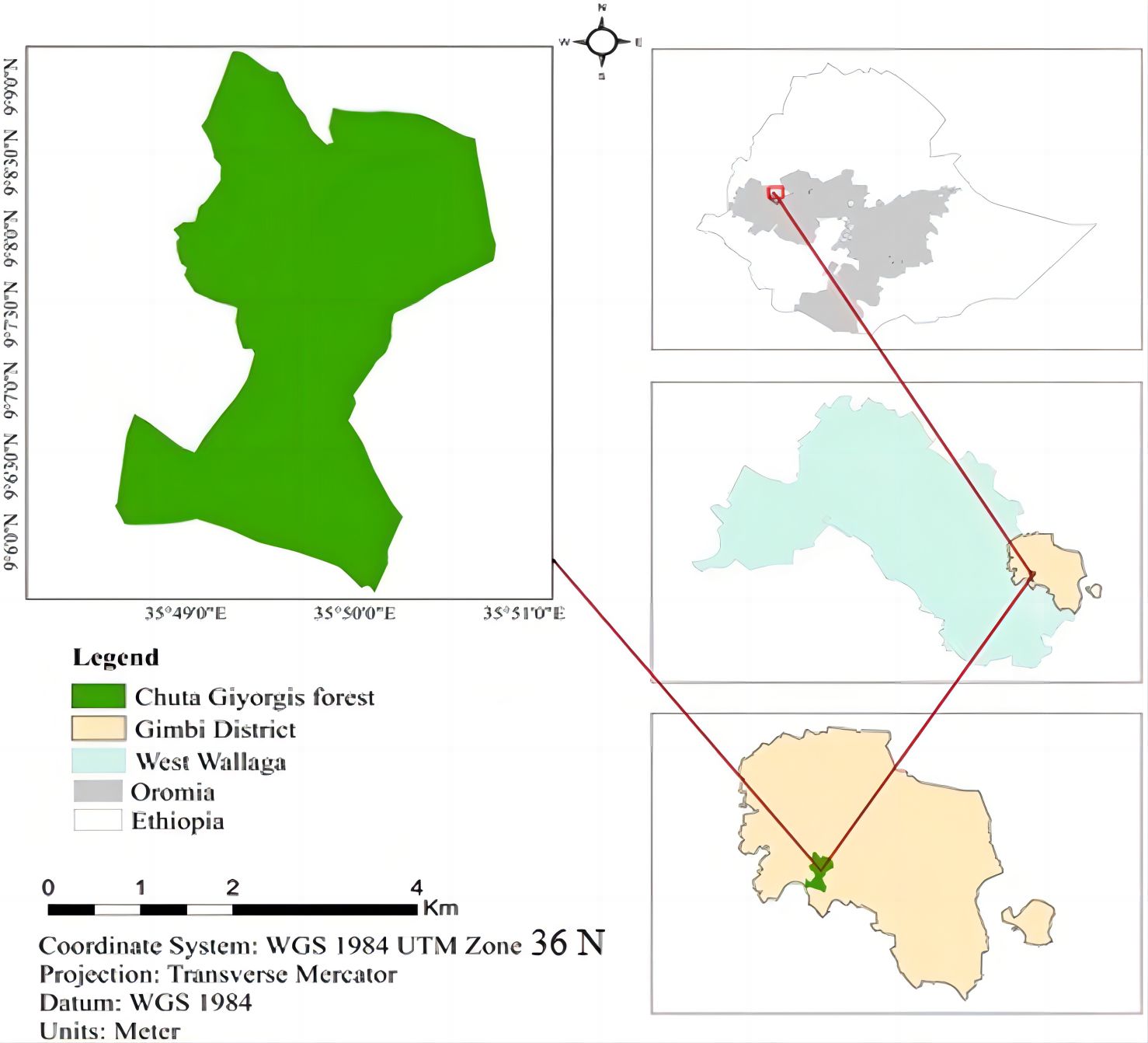
Figure 1. Study area map.

 

2.2 Materials

In this study, various types of primary and secondary data, and software like ArcGIS 10.8, ERDAS IMAGINE 2015, and TerrSet 2020 were used to achieve the research objectives. The primary data types that were used in this study include satellite image, NDVI, and ground control point (GCP) data collected for field verification. Satellite imageries and ancillary data were downloaded freely from the USGS website to identify successive forest cover changes. Secondary data sources like documents, journals, and books were collected from various published and unpublished sources. Background information on the study area was obtained from previous research works in the study area and annual reports of various departments of the West Wallaga zone. The study area boundary was obtained from the Central Statistical Authority.

 

The image data that were used for this study include Landsat 4 (1983), Landsat 7 ETM+ (1991), & Landsat 8 OLI/TIRS (2023) (Table 1). The year 1983 GC was considered because; it was the year when the Chuta Gorgis forest plantation was started. The year 1991 GC, was selected because during this year Dergue regime fell, and due to the fall of this Dergue regime no attention was given to the protection of this forest and as a result, it became deforested at an alarming rate by various factors. The year 2023 was chosen to find updated information about current LULC types and to know the status of this forest at the present.

 

Table 1. Satellite Image Data

 

2.3 Methods

2.3.1 Image Preprocessing

After the Landsat data used was determined, preprocessing of the image like atmospheric correction (cloud and haze removal), geometric correction (nearest neighbor resampling), image enhancement (histogram equalization), band combination (layer stacking), subsetting area of interest were taken place. The image processing task was carried out using Earth Resource Data Analysis System (ERDAS Imagine 2015) software. A land cover map was prepared after the images were downloaded, projected, and layer stacked (pre-process) to be displayed in the ERDAS IMAGINE software interface[18]. Landsat imageries of three bands (4, 3, and 2) for Landsat 4 TM, and Landsat 7 ETM+ whereas bands (5, 4, and 3) for Landsat-8 OLI were used as band combinations in image enhancement to identify changes in land use/land-cover features. These all-mentioned activities were carried out to improve the visible interpretability of an image by increasing the apparent distinction between the features in the scene. The acquired data from the different sources were adjusted to the Ethiopian projection system which is Universal Traverse Mercator Zone 36.

 

2.3.2 Image Classification

The objectives of image classification procedures are to automatically categorize all pixels in an image into LULC classes[19,20]. In this study, supervised classification was carried out to produce five land-use/land-cover classes in the study area (Table 2). In supervised classification user selects an area in the image that represents each unique class and pixel values for each band were recorded for each class. The computer matches the rest of the pixels to user-defined classes. Supervised classification needs the analyst to select training areas where he/she knows what is on the ground and then digitize a polygon within that area. The most commonly used supervised classification is the maximum likelihood classification (MLC) algorithm, which assumes that each spectral class can be described by a multivariate normal distribution[21].

 

Table 2. LULC Classification Scheme

 

2.3.3 Change Detection

According to Lillesand et al.[20], change detection involves the use of multi-temporal datasets to discriminate areas of land cover change between dates of imaging. Although, change detection is useful in such diverse applications as land use change analysis, monitoring of shifting cultivation, assessment of deforestation, seasonal changes in pasture production, damage assessment, disaster monitoring, day/night analysis of thermal characteristics as well as other environmental changes[22]. To perform forest change detection, post-classification change detection comparison methods were employed. To improve the classification accuracy, a post-classification comparison was performed and the classes with mixed pixels were re-examined[23,24].

 

Post-classification was used to examine the forest cover change detection and the rate of its change. This kind of change detection method identifies and provides where and how much change has occurred. In this study, three dates of satellite imageries were used to determine the change by generating quantitative information on spatial and temporal distribution. In the meantime, three aspects of forest cover change detection characteristics such as detecting the changes that occurred, measuring the areal extent of the change, and assessing the spatial pattern of the change were investigated.

 

2.3.4 Ca-Markov Model

To forecast future change, the Markov model simulated variations in LULC over time. The transition area matrix, shows the total area (in cells) expected to change from one LULC class to another over the specified number of time units, and the transition probability matrix, represents the probability that a pixel of a given class will move to another cell class in the next period, were produced using TerrSet's built-in Markov chain analysis module. The likelihood of moving each LULC category to a different category is expressed in a text file as the transition probability matrix, and the number of pixels needed to transition from one LULC class to another over a given amount of time unit is expressed in a text file as the transition area matrix (Figure 2).

 

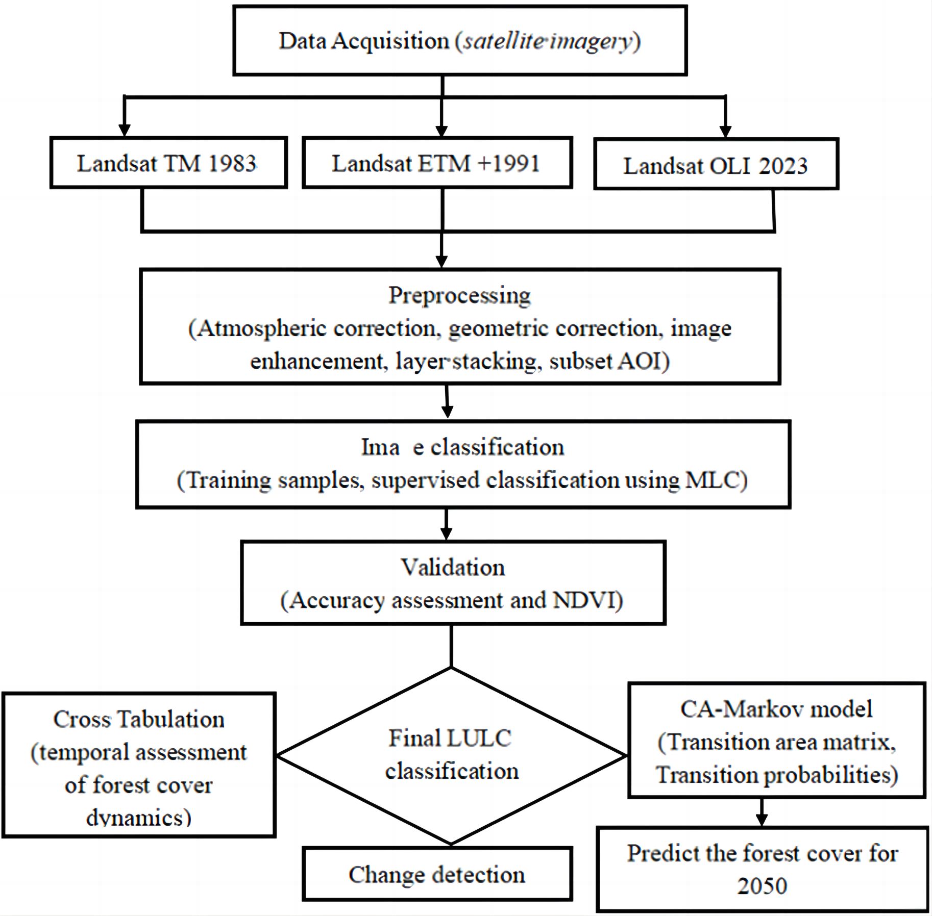
Figure 2. Methodological flowchart.

 

For simulating and forecasting LULC types, CA-Markov is a reliable model that has performed better than alternative approaches[11,25,26]. As a result, the CA-Markov model was employed in this work to simulate and forecast changes in forest cover. The steps in this process were as follows: (i) Markovian chain analysis was performed on the LULC maps from 1983 and 2023 to generate transition area matrices; (ii) creating transitional area maps of LULC change; (iii) evaluating temporal-based forest cover change with the aid of crosstabulation assessment; and (iv) assessing spatial trends of forest cover change and predicting the spatial distribution of LULC in 2050.

 

2.4 Validation

Accuracy assessment and NDVI were employed to validate the image classification result. Before classification data can be used to reliably identify changes, classification accuracy must be evaluated[13]. Accuracy assessment was carried out on the resulting classified imagery using an error matrix and kappa index[27-29] to test the precision and accuracy of imagery and compare them with actual points from the field supplemented by 50 systematic GCPs from high-resolution Google earth data. The Kappa index generates kappa coefficient statistics, the values of which range between 0 and 1. Accordingly, the kappa coefficient (khat) was calculated using the following Equation (1);

 

 

Where TSP = Total sampling point, TCSP = Total correcting sampling point, P = producer/ground truth total, U = user/classified total.

 

Normalized Difference Vegetation Index measures the abundance and growth conditions of vegetation. For vegetated areas, NDVI is high; for non-vegetated areas, NDVI is low. Various mathematical combinations of the Landsat channel 3 (Red band) and channel 4 (NIR band) data are found to be sensitive indicators of the presence and condition of green vegetation. The absolute value of NDVI for vegetation change analysis is between 0 and 1. However, the value of NDVI ranges from -1 to +1. The NDVI empirical analysis is computed using the following Equations (2) and (3):

 

 

 

Where, NIR=Image of Near-Infra Red, and R= Image of Red.

 

3 RESULTS

3.1 LULC Classification

Multispectral and multisensory Landsat images of three consecutive years (1983, 1991, & 2023) were used to evaluate forest cover changes in Chuta Giyorgis. The images were classified into five land cover classes these are, agriculture, bare land, forest, grassland, and water body (Figure 3). In addition, the statistics of LULC change in general and forest cover change, in particular, were computed. The areal extent of each LULC type with the respective percentage is presented in (Table 3).

 

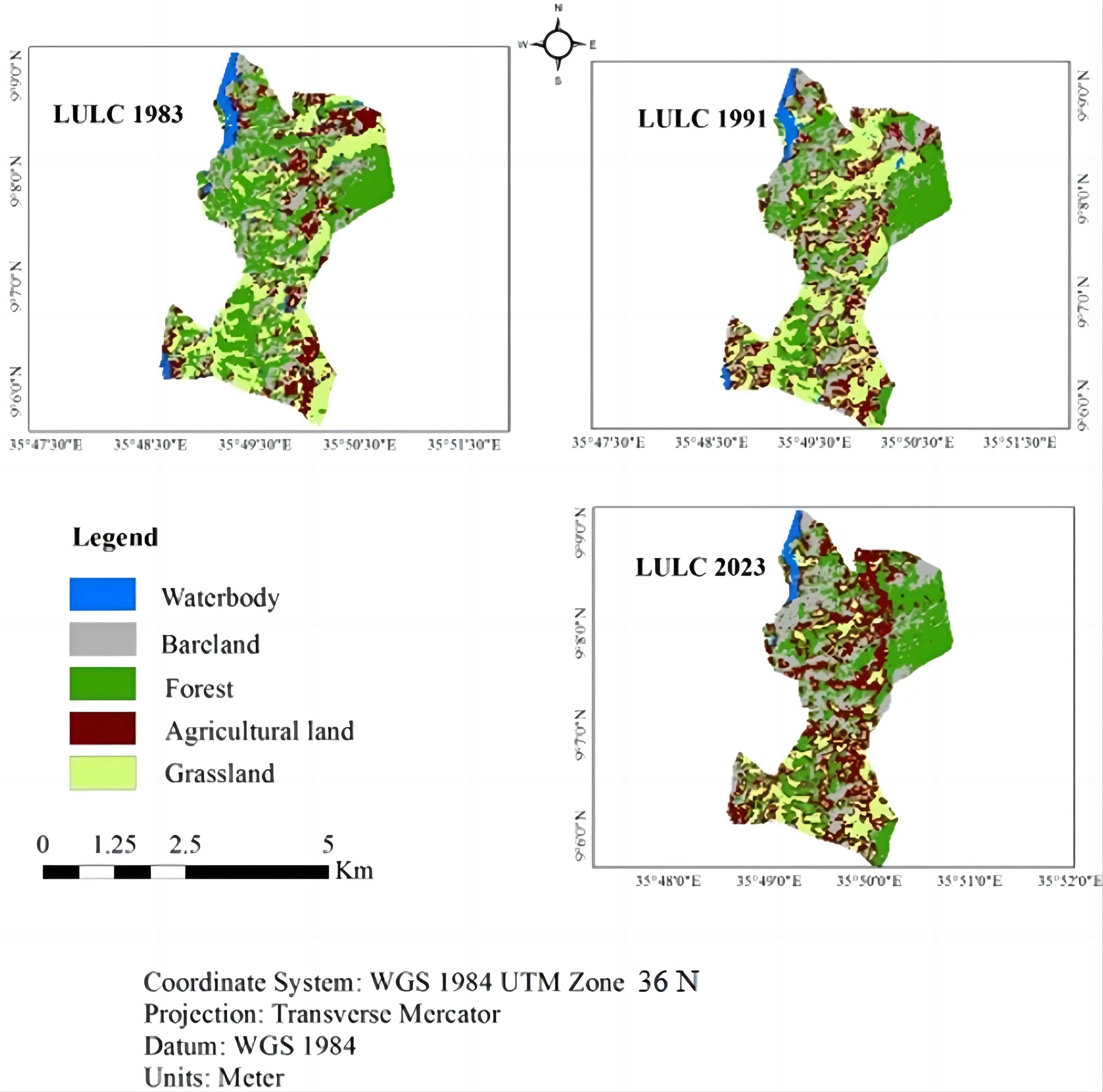
Figure 3. LULC map of 1983, 1991, and 2023.

 

In the first study period (1983), the landscape was dominated mainly by forest lands that covered almost 37.18% followed by grasslands (24.59%), agricultural land (17.66%), bare land (16.47%), and water body (4.10%). Likewise, in 1991 forest land (32.49%) and grassland (25.71%) were the highest coverage of the total area of the study area followed by agricultural land (21.1%), bare land (17.95%), and water land (2.75%). In the last study period (2023), 31.22% of the study area was under agricultural lands, while the share of forest lands (31.07%), bare land (21.39%), grassland (13.79%), and water bodies (2.53%).

 

Table 3. LULC Areas during 1983, 1991, and 2023

Notes :Source: Classified images of 1983, 1991, and 2023

 

3.2 Classification Accuracy

The results of the producer’s accuracy showed that grassland and water bodies have been correctly classified: 89.9%, 95%, and 99% in 1983, 1991, and 2023 respectively. This means that 89.9%, of ground grassland pixels in 1983, 95% of groundwater body pixels in 1991, and 99% of groundwater body pixels in 2023 also appear on the classified images. The lowest producer accuracy was for agricultural land (77.32%, 48.5%, and 78.6%) respectively in 1983, 1991, and 2023. Whereas, results of user’s accuracy presented that in 1983 the maximum class accuracy was for grassland (94.7%) while for the years 1991 and 2023 water bodies had maximum user accuracy of 95% and 100% respectively. This means that approximately 95% and 100% of water body ground truth pixels also appear as water body pixels in the classified image. But for the year 1983 grassland has the highest value of user accuracy (94.7%) which means 94.7% of grassland ground truth pixels also appear as grassland pixels in the classified image. The minimum value of user accuracy was for bare land and agricultural land (75%), bare land (67%), and agricultural land (86.5%) respectively for the years 1983, 1991, and 2023 (Table 4).

 

Table 4. Accuracy Assessment Results for the Years 1983, 1991, and 2023

Notes: Source: From classified images of 1983, 1991, and 2023

 

The overall accuracies for the three reference years (1983, 1991, and 2023) were 83.47%, 81.6%, and 91.4% respectively. This meant that 83.47%, 81.6%, and 91.4% accuracies of the entire classified images also appeared in the classes present in the classified images of 1983, 1991, and 2023 respectively. The Kappa statistics values for the images of the years 1983, 1991, and 2023 were 0.79, 0.77, and 0.89 respectively (Table 4).

 

NDVI assessment can prove where vegetation coverage is highly observed. Accordingly, the values of NDVI were dramatically decreased between the years of 1983-2023. It is important to note that NDVI images were used to measure the balance between energy received and energy emitted by objects on the earth's surface. The NDVI value for the year 1983 ranges from 0.01 (low) to 0.65 (high), 0.06 (low) to 0.58 (high) for the year 1991, and -0.3 (low) to 0.40 (high) for the year 2023, respectively. The Normalized Difference Vegetation Index (NDVI) value between the years 1983 and 2023 was significantly decreased indicating that vegetation cover in the study area was highly disturbed and reduced. Subsequently, Chuta Gorgis forest was converted to other LULC types as was observed from the values of NDVI for the years 1983, 1991, and 2023 (Figure 4 and Table 5).

 

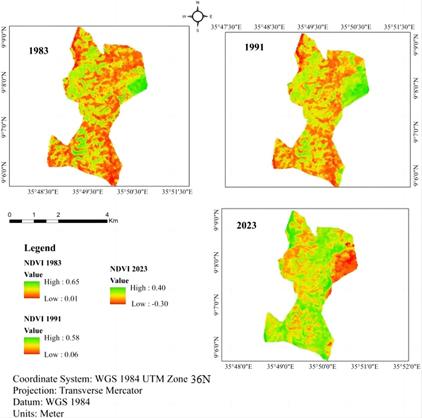
Figure 4. Normalized difference vegetation index maps of 1983, 1991, and 2023.

 

Table 5. Statistics for Normalized Difference Vegetation Index Analysis

Notes: Source: Derived from NDVI map of the years 1983, 1991, and 2023

 

3.3 Change Detection

Land cover change analysis by the post-classification method in this study revealed twenty types of changes between the starting (1983) and ending (2023) periods (Figure 5). In this post-classification activity, the areas that remained unchanged were not considered because the focus was given on the conversion of one land cover type to another for this study. Changes from agricultural land to agricultural land, forest to forest, bare land to bare land, water body to water body, and grassland to grassland were not considered because they were taken as areas not changed. All the changes were analyzed and their area coverage in hectares was also computed (Table 6).

 

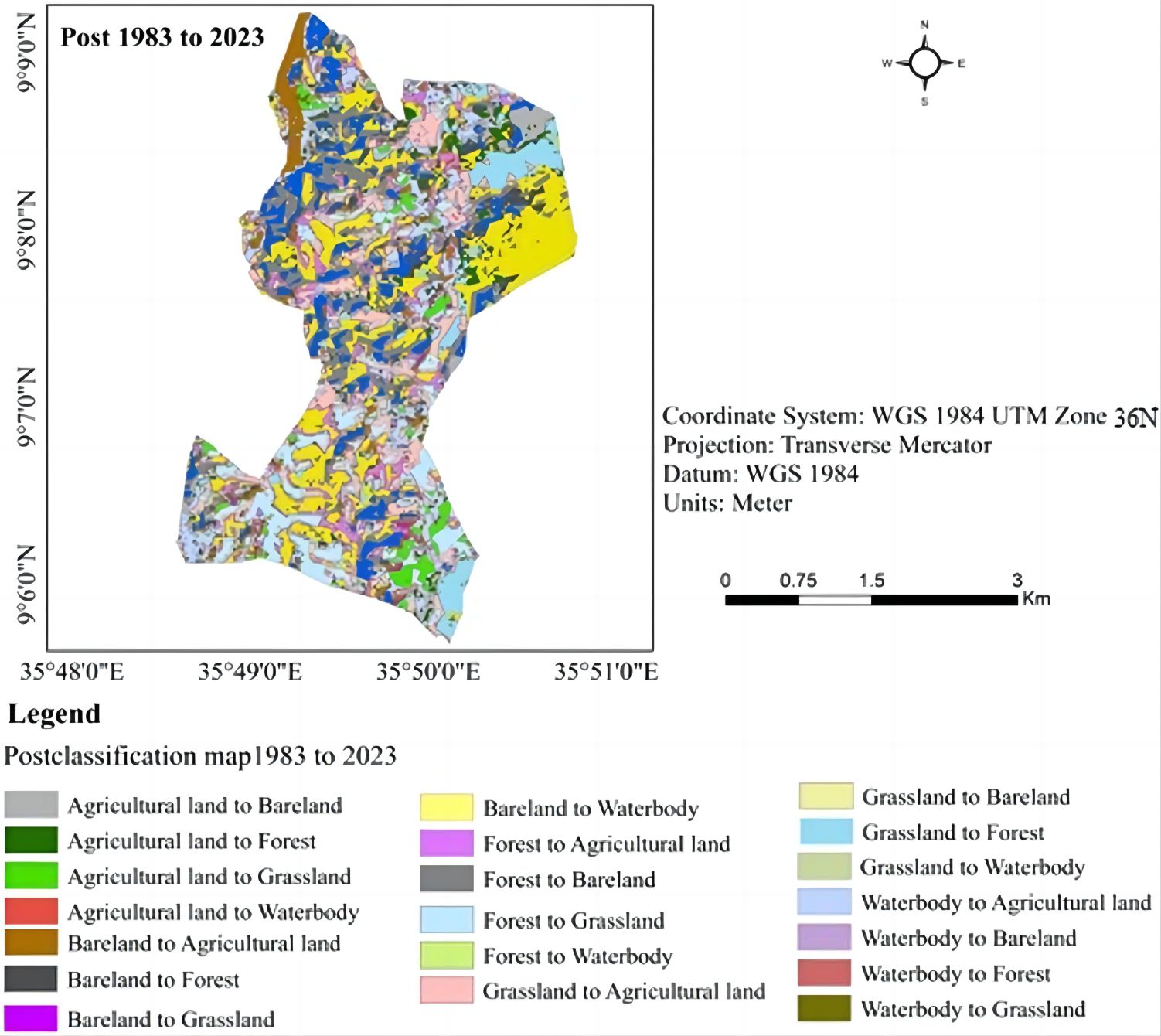
Figure 5. Major LULC conversions took place in the Chuta Gorgis forest from 1983 to 2023.

 

Table 6. Changes Detected from 1983 to 1991, 1991 to 2023, and 1983 to 2023

Notes: NB: AL= Agricultural Land, BL= Bare Land, GL= Grass Land, F= Forest, WB= Water Body. Source: From classified images of 1983, 1991, and 2023

 

Table 6 below shows a summary of the major LULC conversions that have taken place from 1983 to 2023 in the study area. Accordingly, forest land made the highest conversion of 84 ha to bare land in the year from 1983 to 1991 representing a large conversion in the year. From the year 1991 to 2023 grassland made the highest area of conversion 171ha to agricultural land. For the years 1983-2023 grassland made the highest conversion of 138 ha to agricultural land that covered the majority of conversion taking place from the year 1983-2023. The conversion of forest land to bare land during the years (1983-2023) was due to some driving forces which caused deforestation in the area. Yet, some of the forest lands in the initial period were unrestricted and transformed into other LULC classes during each year. On the other hand, there is no conversion occurred from bare land to water body in all three years, and forest to the water body in the years from 1991 to 2023 and 1983 to 2023. Similarly, no conversion has taken place from water bodies to bare land. Other LULC conversions were also observed within a given hectare.

 

3.4 Spatiotemporal Forest Cover Dynamics

The spatial and temporal dynamics of LULC classification were addressed in this portion. Cubic trend surface analysis was computed for the time intervals of 1983-1991, 1991-2023, and 1983-2023 to identify the spatial trends of change for the significant transitions from forest cover to other classes (Figure 6). Spatially, on the northwest and south of the study area, forest cover classes were converted to bare land and settlement respectively, while on the central part, it was highly converted to agriculture, and water in the years 1983 to 2023. Between 1983 and 1991, 1991 and 2023, the change from forest to barren was highly observed in the northwest portion of the study landscape whereas the change from forest to waterbody was the lowest (Table 6 and Figure 6).

 

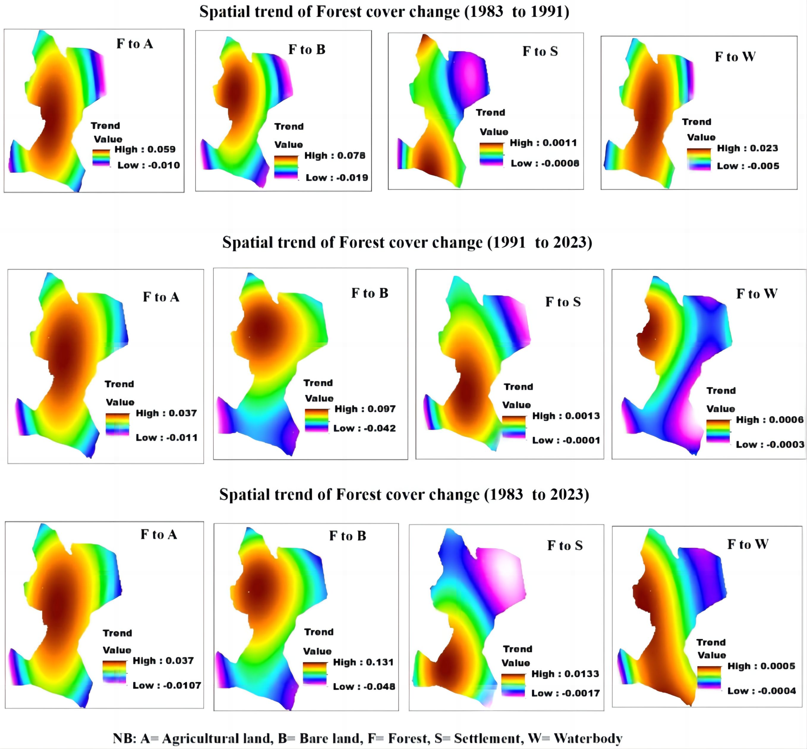
Figure 6. Spatial trend of forest cover change.

 

To extend our understanding of the evolving nature of the LULC types in the Chuta Giyorgis, we applied crosstabulation analysis for changes in 1983 and 2023 (Table 7). All persistence pixels are presented diagonally in bold fonts. The details of the land cover transition between the five land use types are mapped in Figure 7. The corresponding transitional probability matrix and transitional area matrix were also tabulated in Table 8. During the study period, the probability of forest area transitioning into waterbody is very low (0.0007ha) whereas, forest to bare land is the highest transition with 0.1969 hectare.

 

Table 7. Gains/Losses and Persistence of Forest Cover Area (ha)

 

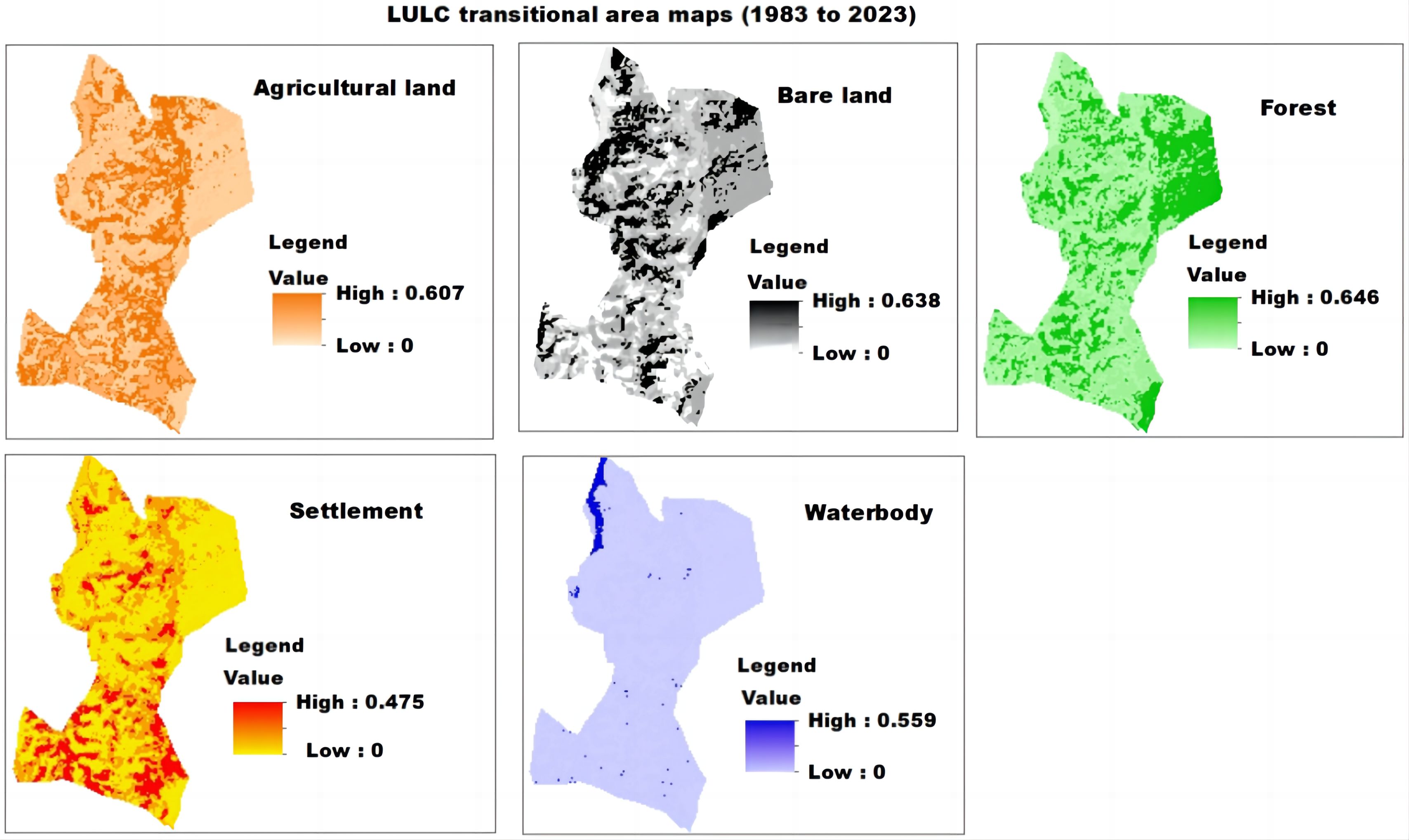
Figure 7. Transitions area map.

 

Table 8. Transition Area Matrices

 

The cross-tabulation analysis was done to explain the losses, gains, and persistence in LULC types during 1983-2023 (Table 9). Forest land has the highest persistence of 261.54ha. Most of the forest land was changed into settlement land (Figure 6). Among all land cover classes, Forest land experienced the maximum amount of total change (234ha) due to its larger areal changes to other classes while water land (28ha) has the least total change (Table 6).

 

For forest land, the amount of area lost (234.54ha) to other classes is more than the amount of area gained (178.02ha) from other classes during 1983-2023 (Figure 8 and Table 8).

 

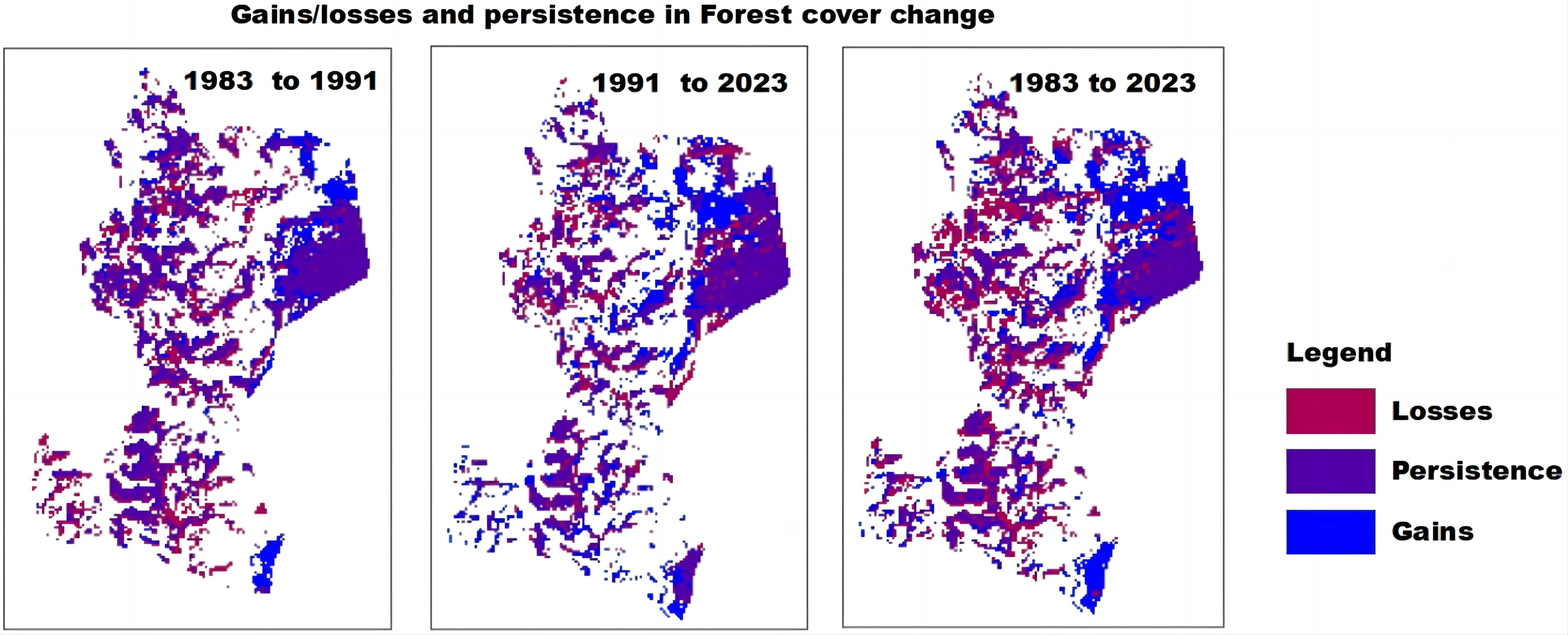
Figure 8. Map of gains, losses, and persistence of forest cover.

 

The spatial and temporal changes in each land cover type obtained from cross-tabulation and trend surface analysis provided the details of a substantial conversion of LULC change that can describe the forest cover dynamics from 1983 to 2023 (Figure 6 and Table 9).

 

Table 9. Cross-tabulation of LULC Types

 

3.5 Prediction of Forest Cover Dynamics

Results of LULC prediction using CA-Markov analysis are shown in Figure 9 and Table 10. Predicted figures for 2050 show the forest cover decreased by 31 hectares (Table 10). Figure 9 shows the predicted spatial destruction of forest cover in 2050. Spatially, forest cover is fragmented with larger patches remaining mainly in the Northeast and south of the Chuta Giyorgis forest while small and narrow patches of forests are also seen scattered in the central part (Figure 9).

 

Table 10. Forest Cover Change Area in Hectares

 

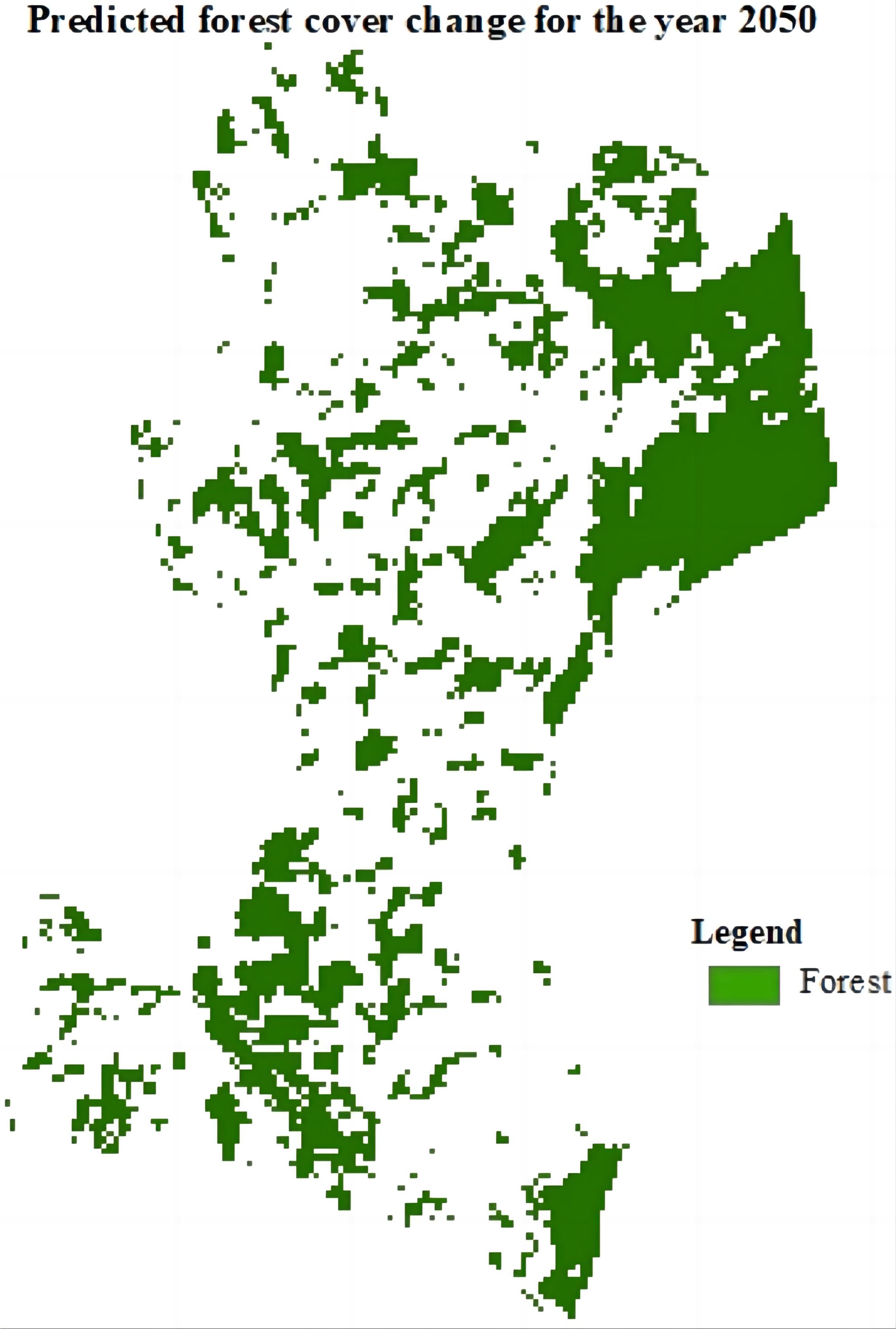
Figure 9. Predicted forest cover map of chuta giyorgis in 2050.

 

4 DISCUSSION

The study used geospatial techniques and CA-Markov models to achieve the research objectives. To produce LULC classification using MLC, assessing the accuracy of classified images, change detection analysis, and NDVI computations were done by geospatial techniques. Whereas, the CA-Markov model was used to assess spatiotemporal forest cover dynamics from 1983 to 2023 and predict forest cover dynamics by 2050 in Chuta Gorgis Forest. For three consecutive years (1983,1991, 2023) LULC of the study area was classified into five classes (Figure 3). The LULC classification was validated using NDVI (Figure 4 and Table 5) and accuracy assessment (Table 4) methods. All of the kappa index values in Table 4 for this particular investigation are greater than 77 percent, indicating good agreement between the observed and projected LULC maps. A Kappa statistics score between 0.60 and 0.80 indicates a significant agreement and a value greater than 0.80 (eighty percent) indicates a good agreement[30]. Similarly, the NDVI outcome showed a progressive shift in the forest cover from the chosen benchmark year to the current date (Table 5). As a result, the maps met the accuracy requirements for the change detection study[31], and the remotely sensed classed samples and the reference data showed a positive association. One of the most used methods for change detection is post-classification[22,32,33]. Throughout the study periods, forest land has been shifted to other LULC classes. However, the overall (1983 to 2023) change detection result shows majority of forest land (127ha) has been converted to bare land (Table 6).

 

Human habitation and its surroundings led to a significant decrease in forest cover and the replacement of LULC types, including grassland, settlement, bare land, and agricultural land which leads to drought and desertification[34-36]. LULC transition map depicts, forest cover is the highest transited class to other classes (Figure 7). The result of spatiotemporal forest cover dynamics shows that the bare land class shared the largest area conversion of forest land than other classes (Table 7). This was due to, the growth of the population in the study area, increased agricultural land demand, and deforestation. Likewise, man-made factors like urbanization, agricultural practices, tree removal for construction, wood, charcoal, furniture, and new grazing areas are contributing to the decline in forest land. This research shows an increase in bare land and agricultural land, leading to the clearing of the area's forest in line with what other experts have reported[12,37,38].

 

The past, present, and future LULC classification results generally show that there was a dramatic loss in forests and a rise in agricultural, settlement, and bare land as a result of anthropogenic and natural factors. The work of several scholars[39-41] studies on LULC change in developing and developed countries prove that the expected patterns of forest cover gradually or quickly transferred to other significant land types. Consequently, the work of these scholars encouraged our results. Within a century, Ethiopia's forest cover decreased from 40% to 3%, according to Desta and Tulu (2015). The study conducted in Ethiopia by Yismaw et al.[42] and Destaab&Tulubc[43] also showed that forest decreased from 40 percent to 3 percent which is in line with the result of our work. Generally, to effectively conserve forests, it may be necessary to inform the government and conservation authorities about the need to amend the preservation action plan.

 

5 CONCLUSION

The study analyzed forest cover changes in the Chuta Giyorgis forest, Oromia region, using CA-Markov and geospatial techniques. Over 40 years, the CA-Markov approach predicted future changes, while the MLC algorithm identified LULC alterations. The study revealed dynamic transformations influenced by natural processes and anthropogenic activities. The study also provided data on the historical and current distribution of forest areas, identifying significant regions and guiding conservation decisions. The study used CA-Markov modeling to analyze vegetation cover in a region, revealing a significant decrease in vegetation. The region currently has only 417ha (31.07%) of forest cover, with significant conversions between 1983 and 2023. By 2050, forest cover is predicted to decrease to 386ha (28.76%), resulting in a fragmented landscape. Forest cover loss threatens ecological functions, increasing vulnerability to erosion, landslides, water scarcity, air pollution, and wildlife extinction. CA-Markov and Geospatial techniques can aid in modeling land use changes, guiding land management, and improving environmental management. The study recommends the implementation of policies based on ecosystem adaptability and other legislative frameworks to maintain the current forest cover and improve the quality of green spaces. Future research endeavors should focus on refining the model, incorporating more precise data sources, and enhancing its predictive capabilities to improve the reliability of forecasts.

 

Acknowledgements

Before anything else, we would want to express our gratitude to God for providing us with the health, peace, knowledge, and wisdom needed to complete this task. We gratefully acknowledge Wallaga University for providing resources, and instrument support for this study.

 

Conflicts of Interest

There is no conflict of interest declared by the authors.

 

Author Contribution

Edosa BT contributed to visualization, investigation, conceptualization, methodology, and software development. Nagasa MD handled data curation, wrote the original draft, worked on software, and conducted validation. Both authors contributed to writing, reviewing, and editing the study. Despite this, they both participated in funding acquisition and evenly split the money from the manuscript file. However, Edosa BT was the chief investigator.

 

Abbreviation List

LULC, Land use and land cover

GIS, Geographic information system

 

References

[1] Hailemariam SN, Soromessa T, Teketay D. Land use and land cover change in the bale mountain eco-region of Ethiopia during 1985 to 2015. Land-Basel, 2016; 5: 41.[DOI]

[2] Sharma K, Robeson SM, Thapa P et al. Land-use/land-cover change and forest fragmentation in Jigme Dorji National Park, Bhutan. Phy Geog, 2017; 38: 18-35.[DOI].

[3] Keenan R, Reams G, Freitas J et al. Dynamics of global forest area: Results from the 2015 Global Forest Resources Assessment. Forest Ecol Manag, 2015; 352: 9-20.[DOI]

[4] Food and Agricultural Organization (FAO). State of the world's forests. Forests and agriculture: Land use Challenges and opportunities, Rome, 2016.

[5] Bognetteau E, Haile A, Wiersum KF. Linking forests and people: A potential for sustainable development of the southwest Ethiopian highlands. Ethiopia Addis Ababa, 2007; 36-53.[DOI]

[6] Muhati GL, Olago D, Olaka L. Land use and land cover changes in a sub-humid Montane Forest in an arid setting: A case study of the Marsabit forest reserve in northern Kenya. Glob Ecol Conserv, 2018; 16: e00512.[DOI]

[7] Food and Agricultural Organization (FAO). Global Forest resource assessment. Rome, Italy, 2010

[8] Reusing M. Change detection of natural high forests in Ethiopia using remote sensing and GIS techniques. Int Arch Photogramm Remote Sens, 2000; 33: 1253-1258.[DOI]

[9] Gole TW, Getaneh F. Sheka forest biosphere reserve nomination form. National MAB Committee of Ethiopia. Addis Ababa, Ethiopia, 2011.

[10] Negassa MD, Mallie DT, Gemeda DO. Forest covers change detection using geographic information systems and remote sensing techniques: A Spatio-temporal study on Komto protected Forest priority area, East Wollega Zone, Ethiopia. Environ Syst Res, 2020; 9: 1-14.[DOI]

[11] Mathewos M, Lencha SM, Tsegaye M. Land use and land cover change assessment and future predictions in the Matenchose Watershed, Rift Valley Basin, using CA-Markov simulation. Land-Basel, 2022; 11: 1632.[DOI]

[12] Gaur S, Mittal A, Bandyopadhyay A et al. Spatio-temporal analysis of land use and land cover change: A systematic model inter-comparison driven by integrated modelling techniques. Int J Remote Sens, 2020; 41: 9229-9255.[DOI]

[13] Wang SW, Gebru BM, Lamchin M et al. Land use and land cover change detection and prediction in the Kathmandu district of Nepal using remote sensing and GIS. Sustainability-Basel, 2020; 12: 3925.[DOI]

[14] Abebe YA, Ghorbani A, Nikolic I et al. Flood risk management in Sint Maarten-A coupled agent-based and flood modeling method. J Environ Manage, 2019; 248: 109317.[DOI]

[15] Armenteras D, Murcia U, González TM et al. Scenarios of land use and land cover change for NW Amazonia: Impact on forest intactness. Glob Ecol Conserv, 2019; 17: e00567.[DOI]

[16] Tolessa T, Senbeta F, Kidane M. The impact of land use/land cover change on ecosystem services in the central highlands of Ethiopia. Ecosyst Serv, 2017; 23: 47-54.[DOI]

[17] Yan Y, Mao Y, Li B. Second: Sparsely embedded convolutional detection. Sensors-Basel, 2018; 18: 3337.[DOI]

[18] Jensen J. Introduction to digital image processing: New York,2004.

[19] Rawat W, Wang Z. Deep convolutional neural networks for image classification: A comprehensive review. Neural Comput, 2017; 29: 2352-2449.[DOI]

[20] Lillesand T, Ralph M, Kiefer RW. Remote sensing and image interpretation, 4th ed. John Wiley & Sons: New York,2015.

[21] Asad MH, Bais A. Weed detection in canola fields using maximum likelihood classification and deep convolutional neural network. Inform Process Agric, 2020; 7: 535-545.[DOI]

[22] Shi W, Zhang M, Zhang R et al. Change detection based on artificial intelligence: State-of-the-art and challenges. Remote Sens, 2020; 12: 1688.[DOI]

[23] Rashid B, Iqbal J. Spatiotemporal change detection in forest cover dynamics along landslide susceptible region of Karakoram highway, Pakistan. ISPRS Ann. Photogramm. Remote Sens Spatial Inf Sci, 2018; 4: 177-184.[DOI]

[24] Edosa BT, Nagasa MD. Spatiotemporal assessment of land use land cover change, driving forces, and consequences using geospatial techniques: The case of Naqamte city and hinterland, western Ethiopia. Environ. Challenges, 2024; 14: 100830.[DOI]

[25] Beroho M, Briak H, Cherif EK et al. Future scenarios of land use/land cover (LULC) based on a CA-markov simulation model: Case of a mediterranean watershed in Morocco. Remote Sensing, 15(4), 1162.

[26] da Cunha ER, Santos CAG, da Silva RM et al. Future scenarios based on a CA-Markov land use and land cover simulation model for a tropical humid basin in the Cerrado/Atlantic Forest ecotone of Brazil. Land Use Policy, 2021; 101: 105141.[DOI]

[27] Verma P, Raghubanshi A, Srivastava PK et al. Appraisal of kappa-based metrics and disagreement indices of accuracy assessment for parametric and nonparametric techniques used in LULC classification and change detection. Model Earth Syst Env,2020; 6: 1045-1059.[DOI]

[28] Martínez Prentice R, Villoslada Peciña M, Ward RD et al. Machine learning classification and accuracy assessment from high-resolution images of coastal wetlands. Remote Sens, 2021; 13: 3669.[DOI]

[29] Keshtkar H, Voigt W, Alizadeh E. Land-cover classification and analysis of change using machine-learning classifiers and multi-temporal remote sensing imagery. Arab J Geosci, 2017; 10: 154.[DOI]

[30] Revuelta-Acosta JD, Guerrero-Luis ES, Terrazas-Rodriguez JE et al. Application of remote sensing tools to assess the land use and land cover change in Coatzacoalcos, Veracruz, Mexico. Appl Sci, 2022; 12: 1882.[DOI]

[31] Anderson JR. A land use and land cover classification system for use with remote sensor data. US Government Printing Office: US,1976.[DOI]

[32] Lunetta RS, Elvidge CD. Applications, project formulation, and analytical approach. Remote sensing change detection: Environmental monitoring methods and applications.Taylor & Francis:London, 1998.

[33] Coppin P, Jonckheere K, Nackaerts K et al. Digital change detection methods in ecosystem monitoring: A review. Int J Remote Sens, 2004; 25: 1565-1596.[DOI]

[34] Akbari M, Shalamzari MJ, Memarian H et al. Monitoring desertification processes using ecological indicators and providing management programs in arid regions of Iran. Ecol Indic, 2020; 111: 106011.[DOI]

[35] Ren Y, Liu J, Shalamzari MJ et al. Monitoring recent changes in drought and wetness in the source region of the Yellow River basin, China. Water-Sui, 2022; 14: 861.[DOI]

[36] Ankomah F, Kyereh B, Ansong M et al. Forest Management Regimes and Drivers of Forest Cover Loss in Forest Reserves in the High Forest Zone of Ghana. Int J For Res, 2020;1:14.[DOI]

[37] Hamad R, Balzter H, Kolo K. Predicting Land Use/Land Cover Changes Using a CA-Markov Model under Two Different Scenarios. Sustain, 2018; 10: 3421.[DOI]

[38] Wang SW, Munkhnasan L, Lee WK. Land use and land cover change detection and prediction in Bhutan's high altitude city of Thimphu, using cellular automata and Markov chain. Environ Challenges, 2021; 2: 100017.[DOI]

[39] Huang W, Liu H, Luan Q et al. Detection and prediction of land use change in Beijing based on remote sensing and GIS. Int Arch Photogramm Remote Sens Spat Inf Sci, 2008; 37: 75-82.[DOI]

[40] Han H, Yang C, Song J. Scenario simulation and the prediction of land use and land cover change in Beijing, China. Sustain, 2015;7: 4360-4370.[DOI]

[41] Miheretu BA, Yimer AA. Land use/land cover changes and their environmental implications in the Gelana sub-watershed of Northern highlands of Ethiopia. Environ Syst Res, 2018; 6: 1-12.[DOI]

[42] Yismaw A, Gedif B, Addisu S et al. Forest cover change detection using remote sensing and GIS in Banja district, Amhara region, Ethiopia. Int J Environ Monit Anal, 2014; 2: 354.[DOI]

[43] Destaab MA, Tulubc FD. Mapping of plantation forest in the upper catchment of Addis Ababa. Int J Environ Sci, 2015; 4: 158-165.[DOI]

 

Copyright © 2024 The Author(s). This open-access article is licensed under a Creative Commons Attribution 4.0 International License (https://creativecommons.org/licenses/by/4.0), which permits unrestricted use, sharing, adaptation, distribution, and reproduction in any medium, provided the original work is properly cited.