Nanoscale Physics: Quantum‒classical Mechanics, Egorov Nano-resonance, Theory of the J-band of J-aggregates, and Beyond

 

Vladimir V. Egorov1*

 

1National Research Center “Kurchatov Institute”, Moscow, Russia

 

*Correspondence to: Vladimir V. Egorov, PhD, Professor, National Research Center “Kurchatov Institute”, Branch of the Kurchatov Complex, Department of Crystallography and Photonics, Photochemistry Center, 7A Novatorov Street, Moscow, 119421, Russia; Email: egorovphotonics@gmail.com

 

DOI: 10.53964/id.2025010

 

Abstract

In quantum mechanics (QM) the theory of quantum transitions works only in atomic physics and in the adiabatic approximation (AA) in molecular and chemical physics. To restore the functionality of QM in molecular and chemical physics beyond AA, Egorov is forced to introduce the so-called dozy chaos (DC) into QM. DC is introduced by replacing the infinitesimal imaginary additive in the energy denominator of the total Green’s function of the system with a finite value. As a result, the transition between quantum states taken in AA becomes continuous, and QM itself becomes quantum‒classical mechanics (QCM). In the case of strong DC, QCM leads to the same results as QM. In the case of weak DC, a regular component in the transient state dynamics appears against the background of chaos. The coherent interaction of the regular component in the electron charge motion and the regular component in the reorganization motion of the nuclei in the environment leads to the so-called Egorov resonance (ER). The same chaos can be strong for small molecules (standard optical spectroscopy) and weak for large molecules (photochemistry and nanophotonics). Therefore, ER is also called nano-resonance. ER explains the nature of the well-known narrow and intense optical J-band of J-aggregates of polymethine dyes, discovered by Jelley and Scheibe in 1936. The first explanation of the nature of the J-band was given by Franck and Teller in 1938 based on the Frenkel exciton concept. This article discusses in detail the evolution of theoretical ideas about the nature of the J-band over almost a century of history and provides a deeply reasoned criticism of them. On the basis of QCM it is explained a large number of experimental data on the shape of optical bands in polymethine dyes and their aggregates. The nature of the physical source of life, possible alternative life forms and the idea of living materials are discussed.

 

Keywords: Planck quantum transitions; Egorov quantum‒classical transitions; dozy chaos; shape of optical bands; optical J-band of J-aggregates; absorption and luminescence; Egorov nano-resonance; physical sourse of life

 

1 INTRODUCTION

As is well known, in theoretical physics the applicability range of any physical theory is limited, and quantum mechanics is no exception. Strictly speaking, the theory of quantum transitions in quantum mechanics[1] works only in atomic and nuclear physics. Its performance there is determined by the convergence of a series of the time-dependent perturbation theory. Generally speaking, this series diverges already in molecular and chemical physics. Its convergence here under the conditions of the Born–Oppenheimer adiabatic approximation[2-6] and the Franck–Condon principle[7-10] is obviously not a guarantee of the correctness of the entire currently existing physical picture of molecular and physicochemical transitions, since in reality there is always at least a small deviation from these conditions[11]. Due to the singularity of the time-dependent perturbation theory series, such a small deviation leads in reality, obviously, not to the need to take into account some small corrections, but to the collapse, for example, of the entire existing physical picture of fast vertical electron transitions and the subsequent slow restructuring of a very heavy nuclear subsystem to a new distribution of electron charge. However, in molecular and chemical physics, the existing erroneous theory often agrees well with experiment. A striking example of such agreement is molecular spectroscopy[12-14]. This paradoxical fact indicates that the existing theory, for example, in molecular spectroscopy, is not regular, but only an interpolation theory. We encounter such an interpolation illusion every day in our everyday life when we observe the movement of the Sun across the sky, a movement that does not actually occur.

 

In molecular and chemical physics, the singularity of the series of the time-dependent perturbation theory in quantum mechanics is associated with the singular nature of the joint motion of light electrons and very heavy nuclei in the transient state within the framework of quantum mechanics. This singularity is easily demonstrated in quantum mechanics using the simplest example of a potential box with a moving wall, where the motion of the wall simulates the reorganization of the entire configuration of nuclei that accompanies quantum transitions of an electron[11,15]. In the case of the potential box example, the singularity is eliminated by introducing friction at the base of the moving wall. In the case of molecular and chemical physics, the singularity is eliminated by replacing the infinitesimal imaginary additive iγ in the energy denominator of the total Green’s function of the system with a finite value. From a systematic comparison of theory with experiment it follows that the energy γ significantly exceeds the energy of an vibrational quantum ℏω:γ>>ℏω. This fact means that the energy γ is not the width of the electron‒vibrational energy levels in the transient state. Such a large value indicates the entanglement of the electron and nuclear motions and, as a consequence, the presence of chaos in their joint motion in the transient state. This chaos is called dozy chaos[11,15-17]. The introduction of chaos into quantum mechanics transforms it into quantum‒classical mechanics (QCM), in which the initial and final states in “quantum” transitions are quantum in the adiabatic approximation, and the transient state, due to dozy chaos, is classical. The transitions themselves in QCM are called quantum‒classical transitions (QCT)[11,15].

 

In the case of strong dozy chaos (γ≅E or γ>>E, E is the nuclear reorganization energy), the rates of QCT become dependent only on the initial and final states, and do not depend on the specifics of the chaotic dynamics of the transient state. We have the same result in the standard Franck‒Condon interpolation picture[1]. This fact explains the reason why the erroneous Franck‒Condon picture[7-10] in theory gives a result consistent with experiment, for example, in molecular spectroscopy[12-14].

 

In the case of weak dozy chaos (γ<<E), the rates of QCT become dependent on the specifics of the transient state dynamics, in which a regular component in the joint electron‒nuclear motion arises against the background of chaos. In this case, quantum mechanics becomes inapplicable in theory even as an interpolation tool, and only QCM should be used[11,15].

 

The same dozy chaos can be weak for large molecules, for example, larger than a nanometer, and strong for small molecules, smaller than a nanometer (see below, Section 9). Therefore, quantum mechanics can still be used for small molecules, but for large molecules it is no longer possible, and QCM should be used. Thus, QCM acts as one of the main theoretical foundations of nanophysics, nanophotonics and photochemistry.

 

One of the interesting consequences of QCM under conditions of weak dozy chaos (γ<<E) is such dynamics of the transient state in which the regular component of the nuclear reorganization motion is coherent with the regular component of the electron motion. This new phenomenon is usually called the Egorov nano-resonance[15,18,19]. At present, in photochemistry, the Egorov nano-resonance explains the narrow and intense J-band of J-aggregates,[16-18,20-28] discovered by Jelley[29,30] and independently by Scheibe[31,32] in 1936.

 

At present, QCM is at the initial stage of its development, and it is constructed in its simplest case, namely, in the case of QCM of elementary electron transfers in condensed matter[11]. Mathematical simplification in the theory of electron transfers is associated with the simplicity of the physics of this problem, where the propagator can be taken as the Green’s function of the electron, and local phonons can be neglected and only non-local phonons can be taken into account[11].

 

In our time, QCM in relation to photochemistry and nanophotonics is called upon to play the same important and fundamental role that quantum mechanics was once called upon to play in relation to atomic spectroscopy.

 

Since from a comparison of theory with experiment we have γ>>ℏω (see above)[16-19,33-38], the energy γ is a measure of dynamic or dozy chaos in a transient state and is called the dozy-chaos energy[16,17]. Dozy chaos involves the movements of the electron charge, nuclear reorganization, and associated fluctuations of the electromagnetic field[39,40].

 

Dozy chaos is created by a light and mobile, unlike nuclei, electron[11]. The chaotic dynamics of the electron and nuclei are subject not to quantum, but to quantum–classical mechanics, or, in other words, dozy-chaos mechanics[11]. The electron, creating chaos (dozy chaos), forces the nuclei to shift to new equilibrium positions corresponding to the new distribution of their charges in the new electronic state, turning their oscillatory movements into the translational motion of the center of mass of the nuclear subsystem.

 

The new mechanics – dozy-chaos mechanics or QCM – is based on the well-known theory of multiphonon transitions[3], or in other words, quantum mechanics of condensed matter[41].

 

The physical source of dozy chaos may be the interaction of the electron charge and spin with the inductive field of optical phonons[41]. In the future, this source can be found theoretically within the framework of quantum‒classical electrodynamics, which will be built taking into account relativistic effects in QCM, just as quantum electrodynamics[42-44] was built on the basis of quantum mechanics[1,45] in the past.

 

Singular molecular transitions in quantum mechanics are damped by chaos by replacing the infinitesimal gamma in the energy denominator of the Green’s function with a finite quantity called the dozy-chaos energy γ (see above)[16,17], similar to the damping of a singular “ultraviolet catastrophe” in classical physics by introducing an elementary quantum of action[11,39,41], that is, Planck’s constant ℏ[46]. Unlike the universal constant ℏ, the dozy-chaos energy γ depends on the specific physical system. However, as a comparison of theory with experiment shows, the numerical value of γ is not completely uncertain, but varies approximately from γ≅E (strong dozy chaos) to ℏω<<γ<<E (weak dozy chaos)[16-19,33-38]. According to the aforementioned analogy with the damping of singularities, the Planck action ℏ can be considered as a hidden parameter in classical mechanics, and the dozy-chaos energy γ can be considered as a hidden parameter in quantum mechanics[47].

 

One of the main goals of this review is to systematically discuss QCM as an alternative to quantum mechanics in molecular and chemical nanoscale physics (see below, Sections 2, 4, 5, 8 and 9). Another goal is to demonstrate the important role of Egorov nano-resonance, which follows from QCM, in explaining many experiments with polymethine dyes and their J-aggregates (see below, Sections 11-13, 17 and 18).

 

In Section 3, a standard theoretical approach to explaining the nature of the narrow and intense J-band of J-aggregates based on the Frenkel exciton model is considered. In this approach it is assumed that in the J-aggregate the optical properties of the monomers forming it are leveled. In the approach based on QCM, on the contrary, it is assumed that these properties develop (see below, Sections 11 and 12). In other words, the Egorov resonance already exists in monomers with certain lengths of the polymethine chain (the main optical chromophore) in certain solvents, but it is less significant than in J-aggregates.

 

The exciton approach erroneously assumes that the J-band of J-aggregates can arise for any type of molecule, whereas the experiment shows that the J-band arises only for polymethine dyes. In Section 3, as an example of the erroneous interpretation of the J-band, I present the results of our work on its computer modeling using the highly efficient calculation method proposed by us. A comparison of two fundamentally different physical approaches to explaining the nature of the shape of the optical bands of J-aggregates and a reasoned choice between them, along with a discussion of the foundations of QCM as an alternative to quantum mechanics in molecular and chemical nanoscale physics (see above), is also one of the main goals of this review.

 

Polymethine dyes serve as a basis not only for the formation of J-aggregates but also for dimers, H- and H*-aggregates. An elucidation of the physicochemical nature of these aggregates and the shape of their optical bands is also the aim of this review (see Sections 14 and 15).

 

An important motivation for studying polymethine dyes and their aggregates, and in particular their optical properties, is the fact that they serve as the simplest example of structural‒dynamic self-organization of molecular matter, which may be relevant to the possible discovery of the physical cause of life (Sections 20-22).

 

2 QCM AND NATURE OF THE FRANCK‒CONDON PRINCIPLE

Quantum physics is the basis of new quantum technologies such as quantum computers, high-temperature superconductivity, and quantum cryptography. The creation of new technologies is closely related to the study of the fundamental effects of quantum decoherence[48]. The creation of quantum states, in which decoherence effects are small, is one of the main applied goals of this fundamental research[48]. A major role in these studies and their applications is played by the study of the dynamics of the joint motion of electrons and nuclei during “quantum” transitions in photochemistry and nanophotonics, as well as in all nanophysics and nanoscience[11,15,18-20,47,49].

 

Recently discovered theoretically by Egorov, the new property of the electron to cause chaos (dozy chaos) in the vibrational motion of nuclei, “in order to control” their movements, leads, as a result of dozy chaos, to the appearance of classical elements in the motion of the quantum system “electrons + nuclei” (cf. Section 1). Appearance of classicality effects in the motion of a quantum system is widely discussed in modern physics and chemistry based on various approaches[50-54]. Egorov’s approach[11,15-20,33,34,36-38,47,49] differs from all these approaches. As mentioned above, Egorov’s approach is associated with a new property of the electron, which is expressed in its creation of chaos in the transient state and, along with it, the classical nature of its joint motion with nuclei. Although such a formulation of the problem is not discussed in the existing literature, the relevance of the very formulation in the literature of the question of the presence of classicality effects in a quantum system is beyond doubt, since quantum mechanics itself arose on the basis of classical mechanics, and, by and large, as its development.

 

Indeed, the basis of quantum mechanics is associated with the need to take into account the interaction of a microparticle with a macroscopic classical measuring device[45]. The fundamental dynamical equation, the Schrödinger equation, was postulated by Schrödinger, but was actually derived from the Hamilton–Jacobi equation for the action S in classical mechanics by introducing the wave function in the form[55] now called the semiclassical approximation[1,45]. The width of energy levels[44,56,57], “within which” the energy spectrum is continuous, is a sign of the partially classical nature of the dynamics in quantum systems. QCM, proposed by Egorov[11,15-17,33,37,38,41,47], is not a “mixture” of quantum mechanics and classical mechanics, but includes essentially modified quantum mechanics, in which the initial and final states are quantum in the Born‒Oppenheimer adiabatic approximation, and the chaotic transient state due to dozy chaos is classical (cf. Section 1). The Franck‒Condon principle in molecular physics avoids consideration of the dynamics of a transient state, which is unreasonably considered unimportant. The classicism inherent in quantum mechanics itself is complemented in molecular physics by the classicism associated with the Franck‒Condon principle. It is assumed that the quantum transition (fast vertical jump) of an electron from the ground to the excited electronic state of a molecule occurs between the turning points of classically moving nuclei, where the nuclei are at rest. In fact, the classical nature of motion in molecular physics is associated not with the Franck‒Condon principle, but with the chaotic dynamics of the motion of the electron and nuclei in the transient state, and therefore in standard molecular spectroscopy of small molecules (see Section 1), the Franck‒Condon principle is illusory in nature[47]. So at one time it was a mistake to call it a principle[10], rather than a hypothesis that has found successful application in molecular spectroscopy[12-14] (Compare with a real principle, such as Hamilton’s principle of least action.). The singular nature of the Franck‒Condon principle is discussed in Section 22.5.

 

The analogue of the situation with the illusory nature of the Franck‒Condon principle is well known[47]. It is a clash of two worldviews: geocentric and heliocentric. As you know, the correct worldview is the heliocentric worldview, in which the Earth rotates both around the Sun and around its own axis. However, being on the surface of the Earth, the rotation of the Earth around its own axis is perceived by the observer as the movement of the Sun across the sky, which is adequately modeled by the erroneous geocentric worldview. It is even customary to talk about the time of sunrise and sunset at a given specific point on the Earth’s surface. However, moving away from the Earth’s surface to a sufficiently large distance into space directly shows the fallacy of the geocentric view of the world. In our case, going into space corresponds to the theoretical description of QCT, for example, in photochemistry and nanophotonics of large molecules, as well as in nanoscale physics and nanoscience in general.

 

Currently, QCM and the corresponding physical picture of molecular “quantum” transitions are based on their simplest example, namely the example of QCM of elementary electron transfers in condensed matter[11,41]. It is shown below that the result of QCM of elementary electron transfers in the shape of an optical band in the case of strong dozy chaos coincides with the corresponding result in the shape of an optical band, which is obtained in quantum mechanics using the Franck–Condon principle (see Sections 7 and 9). The fact that the results of QCM in the case of strong dozy chaos in this particular case, that is, in the case of elementary electron transfers, coincide with the corresponding results of standard quantum mechanics is general. This applies not only to the QCM of elementary electron transfers in condensed matter, but also to all QCM in general, which has yet to be created in the future. This conclusion seems obvious when we consider that the transition to strong dozy chaos discussed here is a “long transition” from a very well-organized dynamical system, containing within itself the unique result of a narrow and intense J-band of J-aggregates, to a completely disorganized system. It is clear that such a transition to the limit of strong dozy chaos from a poorly organized dynamic system, represented in standard spectroscopy by relatively small molecules, would occur much more efficiently with intensification of dozy chaos.

 

3 ON THE HISTORY OF THEORETICAL APPROACHES TO EXPLAINING THE J-BAND OF J-AGGREGATES

3.1 Current State of the Theory of the Shape of Optical Bands in Polymethine Dyes and J-aggregates

3.1.1 General Characteristics of the State of the Problem

The shape of the optical bands of polymethine dyes and their J-aggregates has been intensively studied for more than half a century. Great interest in this problem is associated with the unique spectral characteristics of these organic systems, which determine their wide practical application associated with the conversion of light energy. Detailed information about the applications can be found, for example, in recent reviews[27,58]. The chromophores of these polymethine systems have a relatively simple structure. Therefore, these systems can find wide application in the design and development of targeted molecular systems. Relatively narrow and intense bands are observed in their absorption and fluorescence spectra.

 

At low temperatures, the intramolecular vibrational structure of polymethine dye monomers is spectrally resolved. These spectra were first explained on the basis of the theory of multiphonon transitions[3,4] and approximated by a set of Poisson distributions[4]. At high (room) temperatures, the vibrational structure of the spectra of monomers is not resolved and, as at low temperatures, the spectra are asymmetric. At high temperatures, the theory of multiphonon transitions[3,4] gives a Gaussian (symmetric) shape of optical bands, which successfully explains the symmetric optical bands of impurity centers in dielectrics and semiconductors and, accordingly, does not explain the asymmetric optical bands of polymethine dyes. This fact is associated with a strong difference in the electronic structure of the chromophores: in impurity centers this structure is localized, while in the main chromophore of the dye — the polymethine chain — the electronic (π-electron) structure is highly extended. So, the standard theory of multiphonon transitions turns out to be inapplicable to extended electronic transitions in polymethine dyes. The fact that the vibrational structure of the spectra is unresolvable at high temperatures indicates that the shape of the bands in polymethine dyes is determined by the interaction of the electronic transition not with intramolecular vibrations, but with the nuclear environment. Note that in the current phenomenological exciton theory of the J-band of J-aggregates, the properties of the electronic transition in the chromophore of polymethine dye monomers and its interaction with the environment are not discussed at all. In this case, the shape of the optical band of the monomers is roughly assumed to be Gaussian (see below, Sections 3.1.2 and 3.1.3). The asymmetric optical bands of polymethine dyes are also not explained by the well-known phenomenological Kubo’s shape of bands[16,17,59,60], which produces both Gaussian and Lorentzian shapes, as well as a transition from one shape to the other. Thus, the problem of the shape of the optical band of polymethine dye monomers remained unresolved until relatively recently. The same conclusion applies to the problem of the anomalously narrow and high-intensity optical band (J-band) of their J-aggregates, which we will consider below.

 

3.1.2 J-aggregates and the Statistical Exciton Approach

As stated in Section 1, in 1936, Jelley and Scheibe[29-32], by increasing the concentration of polymethine dye (pseudoisocyanine) in an aqueous solution, independently discovered a strong narrowing and red shift of the optical absorption band, as well as a strong increase in its intensity. This optical band is now called J-band after Jelly. The reason for the appearance of the J-band is usually considered to be the occurrence of molecular aggregates of polymethine dyes, the so-called J-aggregates. It is assumed that in J-aggregates, electronic transitions of monomers strongly interact through excitons[61], similar to molecular crystals[62-64]. This hypothesis about the excitonic nature of the J-band, based on Frenkel’s exciton concept[65], is generally accepted[66]. In 1938, Franck and Teller proposed as a model to describe the red shift and intensity enhancement a one-dimensional linear chain of two-level molecules (immersed in a condensed medium) with dipole-dipole interaction, where the dipoles of the electronic transitions are oriented in a head-to-tail manner[67]. In this model, excitonic states are allowed only near the bottom of the exciton band (red shift), and the total oscillator strength of the optical transition is the sum of a large number of monomer oscillator strengths (intensity enhancement). Subsequently, it was studied in detail by Kasha and his co-authors[68-72].

 

In 1984, Knapp, Scherer and Fischer set the problem of quantitatively explaining the shape of the J-band within the framework of excitonic theory based on statistical consideration of the influence of the medium on the positions of the electronic energy levels of molecules coupled by excitonic interaction in the linear chain[73,74]. The statistical disorder is averaged out by the rapid motion of the Frenkel exciton. Disorder and optical bandwidth decrease, roughly speaking, by a factor , where Nc is the number of coherently bound molecules (the effect of narrowing due to excitonic exchange or Knapp narrowing)[73]. Subsequently, within the framework of the Frenkel exciton model, the shape of the J-band was studied in detail by a large number of theorists[75-83], including Egorov and co-authors[16,17,75-78].

 

In Knapp’s work, the narrowing effect due to excitonic exchange was obtained by analytical methods using perturbation theory[73]. However, in the case, for example, when the number of coherently bound molecules is much less than the length of the aggregate, solving the problem using perturbation theory is impossible and requires numerical calculations. Makhov et al.[75-78] carried out a series of works on the numerical calculation of the shape of optical bands of molecular aggregates within the framework of the statistical exciton approach. Further, in Section 3.1.3 we will briefly review these works and the results obtained in them. These issues, like the entire problem of the J-band of J-aggregates, are discussed in detail by Egorov in his studies[16,17].

 

3.1.3 Computer Simulation of the Shape of Optical Bands in Molecular Aggregates within the Framework of the Statistical Exciton Approach

3.1.3.1 Model Description

Within the framework of the statistical excitonic model, dye molecules are considered as simple (structureless) two-level quantum systems with randomly distributed energies of electronic transitions. They are designed to take into account molecular vibrations, inhomogeneous broadening and other factors that determine the optical absorption spectrum of molecules. This model makes it possible to explain the characteristic features of the absorption spectra of J-aggregates, namely the shift, narrowing and asymmetry of the optical band. However, the calculation methods used in the literature have very low efficiency, which leads to strong spurious noise in the calculated spectrum. Thus, there is an obvious need for a highly efficient calculation method that would allow one to obtain fairly accurate spectra at a reasonable cost of computer time. Such a highly efficient method for calculating the shape of optical bands of molecular aggregates was developed in the works of Makhov et al[75-78]. The use of this method made it possible, in particular, to obtain correct dependences of the shape of the aggregate bands on the system parameters.

 

For the statistical exciton model, the Hamiltonian of the aggregate has the form[66,73-76,78,84,85]:

 

$$ H={\sum }_{n}\left|n\right.⟩{\epsilon }_{n}\left.⟨n\right|+{\sum }_{\begin{array}{c}n,m\\ n\ne m\end{array}}\left|n\right.⟩{v}_{nm}\left.⟨m\right|\left(1\right)$$

 

where |n⟩ is the state in which electronic excitation is localized on the nth molecule, εn are the various electronic transition energies, and vnm is the energy of the resonant interaction between the nth and mth molecules. The disorder of the εn transition energies is called diagonal disorder; the disorder of the vnm interaction energies, due to the disorder of the transition dipole moments and intermolecular distances, is called off-diagonal disorder. In most works devoted to the theoretical study of the shape of optical bands of molecular aggregates, they are limited to considering only diagonal disorder, and the values of vnm are considered fixed. In our work we also adhere to this approximation[75-78].

 

The shape of the optical absorption band of molecular aggregates is determined by the expression[66,73-76,78,84,85]:

 

$$ I\left(\Omega \right)\propto \int \dots \int d{\epsilon }_{1}\dots d{\epsilon }_{N}P\left({\epsilon }_{1},\dots ,{\epsilon }_{N}\right)$$

$$ \times {\sum }_{k=1}^{N}{\left|⟨S|{\psi }_{k}\left({\epsilon }_{1},\dots ,{\epsilon }_{N}\right)⟩\right|}^{2}\delta \left({E}_{k}\left({\epsilon }_{1},\dots ,{\epsilon }_{N}\right)-\hslash \Omega \right)\left(2\right)$$

 

where

 

$$ \left|S\right.⟩=\frac{1}{\sqrt{N}}{\sum }_{n=1}^{N}\left|n\right.⟩\left(3\right)$$

 

and P(ε1,...,εN) is the probability distribution for the transition energies of molecules.

 

3.1.3.2 Perturbation Theory and Numerical Calculations

It is known that disorder leads to the localization of the system’s eigenstates (Anderson localization), and the delocalization length tends to infinity as the disorder tends to zero. In the case when the exciton delocalization length is much greater than the length (number of molecules) of the aggregate N, i.e., when the strong inequality holds[73]

 

$$ \left(1/\pi \right){\left(\sigma /v\right)}^{2}{\left(N/2\pi \right)}^{3}\ll 1\left(4\right)$$

 

where (σ⁄v) is the relative disorder, perturbation theory gives the following relation between the half-widths w1 and wN of the optical bands of the monomer and the aggregate[73]:

 

$$ {w}_{N}={w}_{1}/\sqrt{N}\left(5\right)$$

 

If a correlation occurs between the transition energies of different molecules in the aggregate, Equation (5) is replaced by [73]

 

$$ {w}_{N}=\frac{{w}_{1}}{\sqrt{N}}{\left[\left(\frac{1-{\beta }^{N}}{1+{\beta }^{N}}\right)\left(\frac{1+\beta }{1-\beta }\right)\right]}^{1/2}\left(6\right)$$

 

where β is the correlation parameter. When there are no correlations (β=0), Equation (6) becomes Equation (5). With full correlation β→1 the half-width wN=w1.

 

In the opposite case, when the exciton delocalization length is much smaller than the aggregate length N, as indicated above (Section 3.1.2), solving the problem using perturbation theory is impossible and requires numerical calculations.

 

In such numerical calculations, the integral in Equation (2) is usually calculated by the Monte Carlo method with the δ -functions in the integrand replaced by some functions of small but finite width η. However, this calculation method has extremely low efficiency, which usually leads to a high level of noise in the calculated spectrum (see, e.g., Figure 1, which reproduces the experimental data from Fidder H et al.[84]). This is due to the fact that, on the one hand, the parameter η must be small enough for a good approximation of the δ -functions, and on the other hand, integration by the Monte Carlo method requires that in the η-neighborhood of each point Ω a sufficiently large number of eigenvalues of Hamiltonians with random energies εn lie. The simultaneous fulfillment of these two conditions requires the diagonalization of a huge number of random Hamiltonians, which is often difficult to achieve even with the help of modern powerful computers. Makhov et al.[75,78] proposed a mathematical method that allows one to overcome these difficulties and obtain fairly accurate spectra with a relatively small amount of calculations.

 

3.1.3.3 Highly Efficient Method in Numerical Calculation; Gaussian Diagonal Disorder. Calculation Results

Let us first consider the most common case of aggregates with Gaussian disorder:

 

$$ P\left({\epsilon }_{1},\dots ,{\epsilon }_{N}\right)=\frac{1}{{\left(\sqrt{2\pi }\sigma \right)}^{N}}\mathit{exp}\left(-\frac{{\left({\epsilon }_{1}-\hslash {\Omega }_{0}\right)}^{2}+\dots +{\left({\epsilon }_{N}-\hslash {\Omega }_{0}\right)}^{2}}{2{\sigma }^{2}}\right)\left(7\right)$$

 

Let us make the following change of variables in Equation (2)[75]:

 

$$ {\epsilon }_{k}^{\text{'}}={\sum }_{n=1}^{N}{c}_{nk}{\epsilon }_{n}\left(8\right)$$

 

where

 

$$ {c}_{nk}=\frac{1}{\sqrt{N}}\left[\mathit{sin}\left(\frac{2\pi }{N}\left(n-1\right)\left(k-1\right)\right)+\mathit{cos}\left(\frac{2\pi }{N}\left(n-1\right)\left(k-1\right)\right)\right]\left(9\right)$$

 

It can be seen that is the arithmetic mean of all energies εn. Thus, transformation (8) and (9) isolates (up to a constant) the arithmetic mean of all transition energies as one of the new independent variables.

 

Since transformation (8) and (9) is orthogonal, the old variables can be expressed in terms of the new ones:

 

$$ {\epsilon }_{n}={\sum }_{k=1}^{N}{c}_{kn}{\epsilon }_{k}^{\text{'}}\left(10\right)$$

 

Substituting Equation (10) into Equation (1), we divide the Hamiltonian of the aggregate into two parts:

 

$$ H=\frac{{\epsilon }_{1}^{\text{'}}}{\sqrt{N}}+{H}^{\text{'}}\left(11\right)$$

 

Where

 

$$ {H}^{\text{'}}={\sum }_{n=1}^{N}\left|n\right.⟩\left({\sum }_{k=2}^{N}{c}_{kn}{\epsilon }_{k}^{\text{'}}\right)\left.⟨n\right|+{\sum }_{\begin{array}{c}n,m\\ n\ne m\end{array}}\left|n\right.⟩{v}_{nm}\left.⟨m\right|\left(12\right)$$

 

is a reduced Hamiltonian that depends only on the values of ε2',…,εN'. Thus, we separated the fluctuations of the average transition energy from the relative fluctuations of the transition energies of the molecules in the aggregate. Note that this procedure is similar to the usual separation of the motion of the center of mass from the relative motion within a dynamic system. In short, we have moved to a coordinate system with the origin of the energy scale , which fluctuates according to a given diagonal disorder.

 

From Equation (11) it follows that

 

$$ {E}_{k}=\frac{{\epsilon }_{1}^{\text{'}}}{\sqrt{N}}+{E}_{k}^{\text{'}}\left(13\right)$$

 

and

 

$$ {\psi }_{k}={\psi }_{k}^{\text{'}}\left(14\right)$$

 

where Ek' and ψk' are the eigenenergies and eigenwave functions of the Hamiltonian H'. From the orthogonality of transformation (8) and (9) it follows that

 

$$ {\sum }_{n=1}^{N}{{\epsilon }_{n}}^{2}={\sum }_{k=1}^{N}{{\epsilon }_{k}^{\text{'}}}^{2}\left(15\right)$$

 

And

 

$$ \left|\mathit{det}‖{c}_{nk}‖\right|=1\left(16\right)$$

 

Thus, after changing variables (8) and (9), Equation (2) takes the form:

 

$$ I\left(\Omega \right)\propto \int \dots \int d{\epsilon }_{1}^{\text{'}}\dots d{\epsilon }_{N}^{\text{'}}\mathit{exp}\left(-\frac{{{\epsilon }_{2}^{\text{'}}}^{2}+\dots +{{\epsilon }_{N}^{\text{'}}}^{2}}{2{\sigma }^{2}}\right){\sum }_{k=1}^{N}{\left|⟨S|{\psi }_{k}^{\text{'}}\left({\epsilon }_{2}^{\text{'}},\dots ,{\epsilon }_{N}^{\text{'}}\right)⟩\right|}^{2}$$

$$ \times \mathit{exp}\left(-\frac{{\left({\epsilon }_{1}^{\text{'}}-\hslash {\Omega }_{0}\sqrt{N}\right)}^{2}}{2{\sigma }^{2}}\right)\delta \left(\frac{{\epsilon }_{1}^{\text{'}}}{\sqrt{N}}+{E}_{k}^{\text{'}}\left({\epsilon }_{2}^{\text{'}},\dots ,{\epsilon }_{N}^{\text{'}}\right)-\hslash \Omega \right)\left(17\right)$$

 

Since the reduced Hamiltonian (12) does not depend on the variable ε1', its eigenenergies Ek' and eigenwave functions ψk' also do not depend on ε1'. Therefore, in Equation (17) we can analytically calculate the integral over ε1'. As a result, we arrive at the final expression for the shape of the optical band of the aggregate[75]:

 

$$ I\left(\Omega \right)\propto \int \dots \int d{\epsilon }_{2}^{\text{'}}\dots d{\epsilon }_{N}^{\text{'}}\mathit{exp}\left(-\frac{{{\epsilon }_{2}^{\text{'}}}^{2}+\dots +{{\epsilon }_{N}^{\text{'}}}^{2}}{2{\sigma }^{2}}\right)$$

$$ \times {\sum }_{k=1}^{N}{\left|⟨S|{\psi }_{k}^{\text{'}}\left({\epsilon }_{2}^{\text{'}},\dots ,{\epsilon }_{N}^{\text{'}}\right)⟩\right|}^{2}\mathit{exp}\left(-\frac{{\left({E}_{k}^{\text{'}}\left({\epsilon }_{2}^{\text{'}},\dots ,{\epsilon }_{N}^{\text{'}}\right)-\hslash \left(\Omega -{\Omega }_{0}\right)\right)}^{2}}{2{\left(\sigma /\sqrt{N}\right)}^{2}}\right)\left(18\right)$$

 

The (N-1) -fold integral (18) is calculated by the Monte Carlo method. In this case, the values of Ek' and ψk' are obtained by numerical diagonalization of the reduced Hamiltonian (12), which, obviously, requires no more computer time than the diagonalization of the original Hamiltonian (1). In addition, due to the absence of δ -functions in the integrand when calculating using Equation (18), the diagonalization of each random Hamiltonian contributes simultaneously at all frequencies of the band, and not only in small neighborhoods of its eigenvalues, as when using Equation (2) directly. This achieves a significant increase in computational efficiency compared to commonly used methods.

 

The high efficiency of our calculation method is clearly demonstrated in Figure 1[17], where the dashed line shows the spectrum we calculated using Equation (18)[75], and the dots reproduce the computational results of similar studies by Fidder H et al.[84], where the authors used Equation (2), replacing the δ-functions with tall narrow rectangles. It can be seen that although both spectra were obtained by diagonalizing the same number of random Hamiltonians (500), the spectrum we obtained is absolutely smooth, and the spectrum by Fidder H et al.[84] has a high noise level. Thus, the use of our method can significantly improve the accuracy of calculations without increasing the cost of computer time.

 

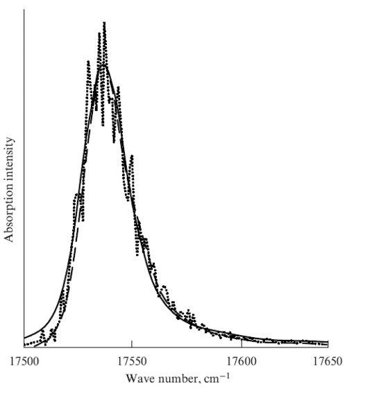
Figure 1. Absorption Band of One-dimensional Aggregates Comprising N=250 Molecules with Gaussian Diagonal Disorder (σ=64cm-1) Taking into Account Resonance Interaction between all Molecules in the Aggregate (V=-600cm-1). Points are numerical calculations by Fidder et al[84]. Dashed line is the results of our numerical calculations[17,75]. Solid line is the experimental absorption band of J-aggregates of pseudoisocyanine bromide[84]. Reprinted (Adapted) from Ref.[17] with Permission from Elsevier B.V.

 

The calculation method based on the choice of a fluctuating energy reference was used for numerical calculations of the optical absorption bands of linear molecular aggregates[75] of various lengths N and flat aggregates with a “brickwork” structure of  molecules in size (see Figure 2), in which the structure parameters q=l⁄h and s ̃=s⁄l vary[77]. For linear aggregates of N=5, 10, 20, 40 and 80 molecules, the relative half-widths of optical bands w ̃N≡wN⁄|v| were calculated as a function of disorder σ ̃≡σ⁄|v| (see Figure 3). The exciton delocalization (coherence) length

 

$$ L=⟨\underset{k}{max}\left({\left|{\mathit{M}}_{0k}\right|}^{2}/{\left|\mathit{M}\right|}^{2}\right)⟩=N⟨\underset{k}{max}\left({\left|⟨S|{\psi }_{k}⟩\right|}^{2}\right)⟩\left(19\right)$$

 

(M0k and M are the transition dipole moments of the kth exciton state of the aggregate and individual molecule, and 〈...〉 means averaging over the ensemble) versus the disorder σ ̃ was also calculated[75]. From Figure 3 it can be seen that at the coherence length L≈1 and the half-width of the aggregate band wN=w1∝σ. The coherence length L increases with a decrease in the disorder . When L<N, half-width and aggregates with different lengths N have bands of approximately equal widths (Figure 3). With a further decrease in the disorder , the coherence length L becomes equal to or greater than the length of the aggregate N, and the result for the half-width of the band , as one would expect, turns into Equation (5) ().

 

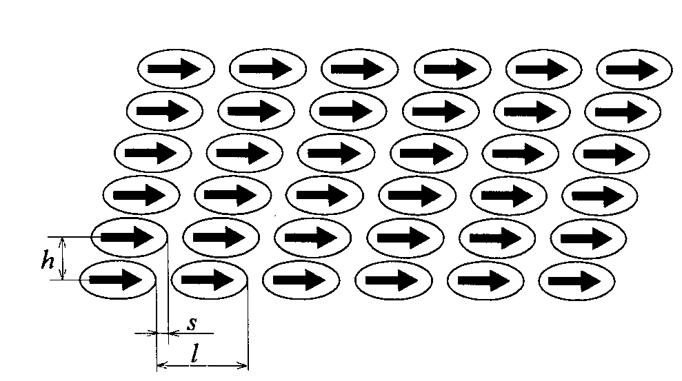
Figure 2. Model Structure for Two-dimensional Moleculer Aggregates in Langmuir Films. Reprinted (Adapted) from Ref.[77] with Permission from Elsevier B.V.

 

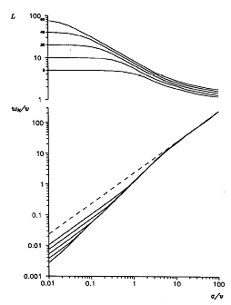
Figure 3. Calculated Dependences of the Relative Absorption Spectrum Half-width wN⁄|v| and Delocalization Length L (Equation (19)) on the Disorder Parameter σ⁄|v| for Cyclic Aggregates Consisting of N=5, 10, 20, 40 and 80 Molecules with Ganssian Disorder. Half-width wN decreases with N. Dashed line is the monomer spectrum half-width. Reprinted (Adapted) from Ref.[75] with Permission from Elsevier B.V.

 

Calculations carried out for two-dimensional aggregates (Figure 2) show that under free boundary conditions, satellite lines appear in the spectrum along with the main line, which at q=7 and reach significant intensity and exceed half the height of the main line[77]. At the same time, under periodic boundary conditions, the absorption band consists of practically one main line. Thus, we can conclude that the appearance of satellite lines is associated with the influence of the aggregate boundary, which, obviously, should be very significant for such small molecular aggregates.

 

Figure 4 shows the dependence we found of the shift of the absorption band , where v0=|M|2⁄h3, on the structure of the aggregate, which, within the framework of the exciton model under consideration, allows us to determine the parameter ranges corresponding to J- and H-aggregates[77]. It can be seen that at , an increase in q leads to a shift of the band to the short wavelength region by reducing the negative interaction between molecules in the chain. An increase in leads to a shift of the band to longer wavelengths. In this case, a maximum appears on the dependence, which then disappears with a further increase in .

 

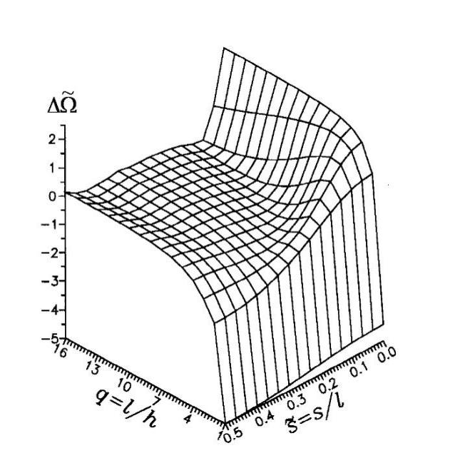
Figure 4. Dependence of the Absorption Spectrum Shift on the Parameters of Structure q=l⁄h and . Reprinted (Adapted) from Ref.[77] with Permission from Elsevier B.V.

 

Note that the highly efficient calculation method we proposed[75] and discussed above (see also below and the next section)[76,78] is known in the literature as the smoothing technique or smoothening technique[79,81].

 

Along with calculation methods based on numerical diagonalization of the Hamiltonian, when calculating the optical bands of molecular aggregates, an approach is often used in which the shape of the band is expressed as the resolvent of the Hamiltonian of the aggregate[73,86]. This approach allows us to avoid the laborious procedure of numerical diagonalization of the Hamiltonian. This advantage is most noticeable in calculations of optical bands for very large aggregates. As in the case of using methods based on numerical diagonalization of the Hamiltonian, the efficiency of calculations using the resolvent of the aggregate Hamiltonian can be significantly increased by using the smoothing technique[76].

 

3.1.3.4 Highly Efficient Method in Numerical Calculation: Arbitrary Diagonal Disorder. Calculation Results

The nature of Gaussian diagonal disorder discussed in the previous section may be related to small molecular vibrations and/or heterogeneity of the local environment. In cases where, for example, the molecules forming an aggregate have several isomeric forms with different transition energies or when the aggregate consists of molecules of several different substances, the probability distribution of transition energies of molecules in the aggregate P(ε1,...,εN) has several maxima. Therefore, the use of Gaussian disorder becomes impossible. For an arbitrary probability distribution P(ε1,...,εN), the new integrand obtained after applying transformations Equation (8) and Equation (9) and subsequent analytical integration over the variable ε1', in comparison with the case of Gassian disorder, will be an extremely complex function of the variables ε2',…,εN' and frequency Ω, which significantly complicates the integration by the Monte Carlo method. To overcome this difficulty, Makhov et al.[78] proposed a more general calculation method as a smoothing technique in which the origin of the energy scale can be chosen so that it fluctuates according to an arbitrary, not just Gaussian, disorder.

 

Let us multiply the integrand in Equation (2) by the following expression, which is obviously equal to one:

 

$$ \frac{\int P\left({\epsilon }_{1}-x,{\epsilon }_{2}-x,\dots ,{\epsilon }_{N}-x\right)dx}{\int P\left({\epsilon }_{1}-y,{\epsilon }_{2}-y,\dots ,{\epsilon }_{N}-y\right)dy}=1\left(20\right)$$

 

where P(ε1-x,ε2-x,...,εN-x) is the probability distribution for the transition energies of molecules in the aggregate, shifted by x in energy and included in Equation (2). Replacing the iterated integral with a (N+1)-fold one, we obtain

 

$$ I\left(\Omega \right)\propto \int \dots \int d{\epsilon }_{1}\dots d{\epsilon }_{N}dx\frac{P\left({\epsilon }_{1}-x,{\epsilon }_{2}-x,\dots ,{\epsilon }_{N}-x\right)P\left({\epsilon }_{1},{\epsilon }_{2},\dots ,{\epsilon }_{N}\right)}{\int P\left({\epsilon }_{1}-y,{\epsilon }_{2}-y,\dots ,{\epsilon }_{N}-y\right)dy}$$

$$ \times {\sum }_{k=1}^{N}{\left|⟨S|{\psi }_{k}\left({\epsilon }_{1},\dots ,{\epsilon }_{N}\right)⟩\right|}^{2}\delta \left(\hslash \Omega -{E}_{k}\left({\epsilon }_{1},\dots ,{\epsilon }_{N}\right)\right)\left(21\right)$$

 

It can be seen that the energy x can be considered, along with the transition energies ε1, ε2, ..., εN, as another random variable over which averaging is carried out. In this case, the function

 

$$ Q\left(x\right)\equiv \frac{P\left({\epsilon }_{1}-x,{\epsilon }_{2}-x,\dots ,{\epsilon }_{N}-x\right)}{\int P\left({\epsilon }_{1}-y,{\epsilon }_{2}-y,\dots ,{\epsilon }_{N}-y\right)dy}\left(22\right)$$

 

in the integrand of Equation (21), depending on ε1, ε2, ..., εN, as parameters, plays the role of a probability distribution for x.

 

Let us choose the value x as the origin of the energy scale. To do this, we will perform a change of variables

 

$$ {\epsilon }_{n}^{″}={\epsilon }_{n}-x\left(23\right)$$

 

It is obvious that the eigenwave functions of the Hamiltonian do not change when the origin of the energy scale is shifted:

 

$$ {\psi }_{k}\left({\epsilon }_{1}^{″}+x,\dots ,{\epsilon }_{N}^{″}+x\right)={\psi }_{k}\left({\epsilon }_{1}^{″},\dots ,{\epsilon }_{N}^{″}\right)\left(24\right)$$

 

$$ {E}_{k}\left({\epsilon }_{1}^{″}+x,\dots ,{\epsilon }_{N}^{″}+x\right)={E}_{k}\left({\epsilon }_{1}^{″},\dots ,{\epsilon }_{N}^{″}\right)+x\left(25\right)$$

 

Thus, from Equation (21) we obtain

 

$$ I\left(\Omega \right)\propto \int \dots \int d{\epsilon }_{1}^{″}\dots d{\epsilon }_{N}^{″}dx\frac{P\left({\epsilon }_{1}^{″},{\epsilon }_{2}^{″},\dots ,{\epsilon }_{N}^{″}\right)P\left({\epsilon }_{1}^{″}+x,{\epsilon }_{2}^{″}+x,\dots ,{\epsilon }_{N}^{″}+x\right)}{\int P\left({\epsilon }_{1}^{″}-{y}^{″},{\epsilon }_{2}^{″}-{y}^{″},\dots ,{\epsilon }_{N}^{″}-{y}^{″}\right)d{y}^{″}}$$

$$ \times {\sum }_{k=1}^{N}{\left|⟨S|{\psi }_{k}\left({\epsilon }_{1}^{″},\dots ,{\epsilon }_{N}^{″}\right)⟩\right|}^{2}\delta \left(\hslash \Omega -{E}_{k}\left({\epsilon }_{1}^{″},\dots ,{\epsilon }_{N}^{″}\right)-x\right)\left(26\right)$$

 

where y″=y-x. Since the quantities Ek and ψk included in Equation (26), the determination of which requires numerical diagonalization of the Hamiltonian, do not depend on the variable x, we can integrate expression Equation (26) over x analytically. As a result, we arrive at the final expression for the shape of the optical band of aggregates in the case of arbitrary diagonal disorder[78]:

 

$$ I\left(\Omega \right)\propto \int \dots \int d{\epsilon }_{1}^{″}\dots d{\epsilon }_{N}^{″}P\left({\epsilon }_{1}^{″},\dots ,{\epsilon }_{N}^{″}\right){\sum }_{k=1}^{N}{\left|⟨S|{\psi }_{k}\left({\epsilon }_{1}^{″},\dots ,{\epsilon }_{N}^{″}\right)⟩\right|}^{2}$$

$$ \times \frac{P\left({\epsilon }_{1}^{″}+\hslash \Omega -{E}_{k}\left({\epsilon }_{1}^{″},\dots ,{\epsilon }_{N}^{″}\right),\dots ,{\epsilon }_{N}^{″}+\hslash \Omega -{E}_{k}\left({\epsilon }_{1}^{″},\dots ,{\epsilon }_{N}^{″}\right)\right)}{\int P\left({\epsilon }_{1}^{″}-{y}^{″},{\epsilon }_{2}^{″}-{y}^{″},\dots ,{\epsilon }_{N}^{″}-{y}^{″}\right)d{y}^{″}}\left(27\right)$$

 

It can be seen that, in contrast to the original expression for the band shape (Equation (2)), the integrand in Equation (27) no longer contains δ-functions, which significantly increases the efficiency of calculations compared to the standard procedure. Another important property of Equation (27) is the fact that the integrand is the product of the normalized function of ℏΩ and the original probability distribution P(ε1″,ε2″,...,εN″), as a result of which the diagonalization of each random Hamiltonian makes an equal integral contribution to the absorption spectrum, thereby ensuring the correct operation of the numerical procedure.

 

Let us illustrate the capabilities of the aforementioned method in the case when the aggregate consists of molecules of two types that differ only in the average transition energy (bi-Gaussian disorder)[17,78]:

 

$$ P\left({\epsilon }_{1},\dots ,{\epsilon }_{N}\right)=\frac{1}{{\sigma }^{N}{\left(2\pi \right)}^{N/2}}{\prod }_{n=1}^{N}\left[b\mathit{exp}\left(-\frac{{\left({\epsilon }_{n}-\hslash {\Omega }_{0}+a/2\right)}^{2}}{2{\sigma }^{2}}\right)\right.$$

$$ \left.+\left(1-b\right)\mathit{exp}\left(-\frac{{\left({\epsilon }_{n}-\hslash {\Omega }_{0}-a/2\right)}^{2}}{2{\sigma }^{2}}\right)\right],a>0,0 < b<1\left(28\right)$$

&nbsp;

Figure 5 shows the results of calculations of the shapes of absorption bands for linear aggregates of N=100 molecules[17,78]. For a symmetric spectrum of a monomer (b=1⁄2, Figure 5A), the inclusion of intermolecular interaction leads to a noticeable asymmetry of the aggregate band already with interaction v⁄a=-0.1. The asymmetry of the band increases with increasing interaction. Ultimately, as in the case of Gaussian disorder, the aggregate band becomes a narrow band with Gaussian long-wavelength and Lorentzian short-wavelength wings. For the asymmetric spectrum of the monomer (b=3⁄4, Figure 5B), a similar picture of changes in the band shape with increasing intermolecular interaction is obtained.

 

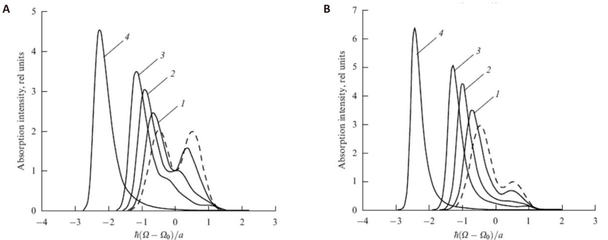
Figure 5. Absorption Bands of One-dimensional Aggregates of N=100 Molecules with Bi-Gaussian Diagonal Disorder (Equation (28)) at the Following Parameter Values: v⁄a=-0.1 (1), -0.25 (2), -0.4 (3), -1 (4); b=1⁄2 (A), 3⁄4 (B)[17,78]. Dashed lines display monomer bands (v=0). Reprinted (Adapted) from Ref.[17] with Permission from Elsevier B.V.

 

Note that introducing the fluctuation beginning of the energy scale is also possible in the case of calculations using the Hamiltonian resolvent[78].

 

3.2 Approach Based on Considering Dynamics of Elementary Excitations of an Extended Electronic System as an Alternative to the Statistical Exciton Approach

As can be seen, we were able to achieve significant progress both in the theory and in its application to explain the shape of the J-band in experiment within the framework of the statistical exciton approach[66,73-78,84,85,87-90]. However, this approach contains significant drawbacks. The key disadvantage of the statistical exciton approach is its inability to take into account the characteristic physicochemical properties of polymethine dye molecules that are part of J-aggregates. It is well known that the chromophore of a polymethine dye is based on a highly extended distribution of electron charge density along the polymethine chain[91-93]. Therefore, any agreement between the existing excitonic approach, no matter what elegant mathematical methods it offers[75,78,87], and experimental data, if this characteristic property of the polymethine dye chromophore is not directly taken into account, can only be considered as curiosity. (It is possible, at first glance, to abandon the use of statistical methods in the exciton approach and thereby improve it using computational methods of quantum chemistry[94]. However, currently existing quantum chemical methods do not allow us to sufficiently fully take into account factors important for extended electronic systems, namely, the effects of coupling between electronic and nuclear motions during electron-phonon transitions.)

 

It is clear that for the success of the theoretical approach, a unified theory is necessary that includes a characteristic property of the π-electronic system — its strong linear expansion — to describe the shape of the optical bands of both J-aggregates and the dye monomers themselves. (Recall that in the excitonic theory, the shape of the optical band of a dye monomer is phenomenologically determined by statistical disorder[66,73-76,78,84,85,87].) Therefore, this unified theory in its simplest form has nothing in common with the theory of excitons[62-64]. In other words, before considering the dynamics of the exciton, it is necessary to study the dynamics of the elementary excitation of an extended electronic system (modeling a π -electron system) interacting with the environment, both in the case of the polymethine chain of the dye monomer and in the case of the J-aggregate, and only after that, if the need arises, it will be possible to raise the question of studying the dynamics of excitons.

 

In short, a theory that claims to explain any property of a complex physical system (the shape of the optical band of J-aggregates), but is unable to explain a similar property of a simpler composite physical element (the shape of the optical band of polymethine dye monomers) cannot be considered satisfactory[15-17]. This fact alone is enough to realize the illusory nature of the exciton approach to the nature of the J-band existing in the physicochemical literature (compare with the illusory nature of the Franck–Condon principle, Section 2). A more detailed criticism of the exciton approach to explaining the nature of the J-band is given below (Sections 3.3 and 3.5). A detailed presentation of the excitonic approach to explaining the nature of the J-band and its detailed criticism in this regard is provided in Egorov’s comprehensive analysis[16,17].

 

3.3 The Born‒Oppenheimer Adiabatic Approximation, the Franck‒Condon principle, and the Statistical Exciton Model of the J-band

The spectra of polymethine dyes at room temperatures are poorly resolved[4] and their shape depends on the interaction of electronic transitions not with the intramolecular vibrations, but with the environment (Section 3.1.1). The interaction of electronic transitions with the environment is described by the theory of multiphonon processes[3]. This theory is based on the Born–Oppenheimer adiabatic approximation and the Franck–Condon principle and gives a Gaussian (symmetrical) distribution for the shape of optical bands at room temperatures (Section 3.1.1). As shown below, the shape of the optical bands of polymethine dye monomers that form J-aggregates is significantly different from Gaussian: it is an asymmetric shape (see below, Section 11). This fact clearly indicates that the solution to the problem of describing the shape of optical bands in polymethine dyes lies beyond the adiabatic approximation and the Franck–Condon principle. Section 11 demonstrates that the new theory — QCM[11,15-17,37,38,47], going far beyond the adiabatic approximation and the Franck‒Condon principle, explains quite well the complex shape of the optical absorption band and its observable variations in the series of the same dye with highly varying lengths of the polymethine chain. In other words, we have convincingly proven that the standard quantum‒mechanical approach, based on the Born‒Oppenheimer adiabatic approximation and the Franck‒Condon principle, cannot be used as a basis for constructing a theory of the shape of absorption bands in polymethine dyes and especially their J-aggregates, due to the highly asymmetrical shape of the J-bands. Meanwhile, the adiabatic approximation and the Franck–Condon principle underlie the statistical exciton theory (Section 3.1.3) of the absorption bands of J-aggregates[16,17]. Therefore, this fact alone does not provide grounds to assert the correctness of the exciton approach to the J-band theory.

 

This brings us to the end of the discussion of the excitonic model. However, a natural question arises: “Why was it used so successfully in the J-band theory?” The obvious answer is: “It assumes a paradigm of static disorder in the electronic energies of molecular transitions in J-aggregates.”

 

The point is that disorder changes significantly as the Frenkel exciton moves along the J-aggregate: some calculations[95] and experimental data[96] show that the characteristic times of disorder change and exciton motion can be of the same order[16]. This puts in doubt[61] the mechanism of exchange narrowing due to the “quickly moving” Frenkel exciton[73] that averages static disorder. In this case, it is necessary to apply exciton models taking into account dynamic disorder[87,89]. However, these models are too complicated and contain many fitting parameters. Under conditions in which the mechanism of exchange narrowing is a priori realizable, an important problem of the degree of disorder correlation between transition energies of aggregated molecules remains open. There is reason to think that it may be very high[97-100]. In such a case, the mechanism of exchange narrowing becomes inefficient, and the J-band is not narrow, but as wide as the optical band of the monomer (Section 3.1.3.2, Equation (6)).

 

Thus, there are two egregious incorrectnesses in the statistical exciton theory of the J-band: the adiabatic approximation with the Franck‒Condon principle and static disorder. It is not unusual in physical chemistry or chemical physics that two incorrect approximations in one theory mutually compensate for each other and yield a result in agreement with experiment. It should be especially emphasized that the very concept of Frenkel excitons is certainly not in doubt. However, its application as it stands to the solution of the J-band problem conceals, even if unintentionally, the errors in the Knapp exciton model[73] and in all later works relying on it[16,17].

 

3.4 The J-band as the Egorov Nano-resonance

We provide an alternative explanation of the nature of the J-band within the framework of a particular and simplest case of QCM, namely within the framework of the QCM of elementary electron transfers in condensed media[11], which includes an explanation of the nature and shape of the bands of polymethine monomers forming J-aggregates[15-17]. As mentioned above, a new explanation of the nature and shape of the J-band is based on the so-called Egorov nano-resonance, discovered in QCM[11,15,18,19,49]. The Egorov nano-resonance is a resonance between the electronic motion and the motion of the reorganization of the nuclei of the environment during quantum–classical transitions in an extended optical chromophore under the condition of weak dozy chaos:

 

$$ {\left(2{\tau }_{e}\right)}^{-1}={\tau }^{-1}\left(29\right)$$

 

where the characteristic time

 

$$ {\tau }_{e}=\frac{L}{\sqrt{2{J}_{1}/m}}\left(30\right)$$

 

(L is the extent of quantum–classical transitions, not to be confused with the exciton delocalization length L in Section 3.1.3.3, Equation (19); J1 is the binding energy of the electron in the initial state 1; m is the effective mass of the electron; cf. below, Section 5) and the characteristic time

 

$$ \tau =\frac{\hslash }{E}\left(31\right)$$

 

(E is the energy of reorganization of the nuclear subsystem, which is half the energy of reorganization of Marcus, see below, Section 5, Equation (44) and Section 7, Equation (87)).

 

Note that the term “Egorov resonance” was introduced by Petrenko & Stein in their article in the ACS journal[18]. Petrenko & Stein[18] also introduced the terms “Egorov’s theory” and “Egorov’s approach”[18]. Following Petrenko & Stein[18], we sometimes use these two short terms in the text below instead of the long term “quantum–classical mechanics of elementary electron transfers in condensed matter”.

 

3.5 Some Remarks on the Problem of the J-Band, and Beyond

At present, a number of researchers[25,27,28,58] continue to adhere to the traditional (exciton) point of view on the nature of the J-band. On the other hand, it should be noted the works of Petrenko & Stein[18,20], which, on the contrary, develop new ideas to explain the nature of the J-band within the framework of QCM[36-38].

 

The recent idea of Guerrini et al. to theoretically explain the nature of the J-band on the basis of plasmon resonance[101] led them to a negative result[15,101].

&nbsp;

Note also that a quantitative comparison of the quantum-classical approach and the excitonic approach (exchange narrowing), to which the reader may a priori call, is impossible. It’s because the excitonic approach, which appeals to an arbitrarily specified static disorder in monomers (diagonal disorder) and appeals to an insufficiently precisely defined value of the exciton interaction (non-diagonal disorder), does not provide such a quantitative explanation in principle. That is, the excitonic approach does not provide a connection between the band shape and well-defined physical parameters of the system that can be measured and/or calculated. For example, the exciton theory (see above, Sections 3.1.2 and 3.1.3) does not include such an important and physically transparent quantity as the nuclear reorganization energy that arises during electronic transitions due to electron‒phonon and exciton‒phonon interactions (see also below, Section 19). The same conclusion also applies, for example, to the Eisfeld–Briggs phenomenological exciton‒vibronic model[80], which is based on the Hamiltonian resolvent method (Sections 3.1.3.3 and 3.1.3.4) and uses the entire experimental spectrum of the monomer as one of the two main parameters of the problem. It is clear that this monomer spectrum, being the basis for the J-band calculation, is uncontrollably modified by monomer interactions within the J-aggregate[16,17]. On the other hand, the quantum-classical approach demonstrates the ability to provide a quantitative explanation of experiment (see below, Section 12).

 

We note that below (Sections 13-18), based on the Egorov nano-resonance, in addition to explaining the nature of the J-band (Section 12), we also explain the experimental J-effects associated with luminescence, which cannot be explained on the basis of the traditional exciton approach (Section 17), as well as effects associated with nonlinear optical absorption in polymethine dyes (Section 18). Section 13 provides an explanation of the dependence of the position of the nano-resonance in the vinylogous series of polymethine dyes on the polarity of the medium. In Sections 14 and 15, taking into account the Frenkel exciton effects in QCM, the position and shape of the optical bands of dimers, H- and H*-aggregates of polymethine dyes are explained. Moreover, the narrow and blue-shifted H*-band of H*-aggregates received its first explanation in the works of Egorov[34,102,103]. Finally, in Section 16, the Petrenko & Stein explanation[20] of a strong detuning of the Egorov nano-resonance as a result of large increase in dye concentration in the Harrison et al. experiment[24] is given.

 

4 MOLECULAR AND CHEMICAL PHYSICS: THE NEED FOR CREATION OF QCM

The theory of quantum transitions in quantum mechanics is based on the convergence of a series of time-dependent perturbation theory (TDPT)[1]. The standard scheme of the perturbation theory is as follows[1]

 

$$ i\hslash \frac{\partial \Psi }{\partial t}=H\left(t\right)\Psi ,H\left(t\right)={H}_{0}+V\left(t\right),V\left(t\right)=\left\{\begin{array}{c}W\left(t\right),\text if\text{0}\text{≤}t\le \tau ,\\ \text{0}\text{,}\text{if} t<0,t>\tau \end{array}\right.\left(32\right)$$

 

The transition amplitude Akl looks like the series:

 

$$ {A}_{kl}\left(t\right)={\sum }_{n=0}^{\infty }\frac{\left.⟨k\right|{I}_{n}\left(t\right)\left|l\right.⟩}{n!}\left(33\right)$$

 

Where

 

$$ {I}_{n}\left(t\right)={\left(\frac{1}{i\hslash }\right)}^{n}P{\int }_{0}^{t}d{t}_{1}{\int }_{0}^{t}d{t}_{2}\dots {\int }_{0}^{t}d{t}_{n}\stackrel{~}{W}\left({t}_{1}\right)\stackrel{~}{W}\left({t}_{2}\right)\dots \stackrel{~}{W}\left({t}_{n}\right)\left(34\right)$$

 

P is the chronological operator of Dyson, and the perturbation operator

 

$$ \stackrel{~}{W}\left(t\right)={e}^{\frac{i}{\hslash }{H}_{0}t}W\left(t\right){e}^{-\frac{i}{\hslash }{H}_{0}t}\left(35\right)$$

 

is taken in the interaction representation. The TDPT series converges in atomic and nuclear physics, as in the matrix elements ⟨k| In (t)|l⟩ (Equation (33)), the states |l⟩ and |k⟩ are regular due to quantum jumps. A small parameter that ensures the convergence of the TDPT series is a small perturbation time τ (see Equation (32)). In the first order of TDPT we have the Golden rule of Fermi[1]

 

$$ {\mathfrak{I}}_{kl}\left(\tau \right)={\left|{A}_{kl}^{\left(1\right)}\left(\tau \right)\right|}^{2}=\frac{1}{{\hslash }^{2}}{\left|{\int }_{0}^{\tau }\left.⟨k\right|\stackrel{~}{W}\left(t\right)\left|l\right.⟩{e}^{i{\omega }_{kl}t}dt\right|}^{2}\left(36\right)$$

 

where ℏωkl=Ek‒El, Ek and El are the energies of stationary states.

&nbsp;

In molecular and chemical physics, the TDPT series converges only in the case of transitions according to the Franck–Condon principle[7-10], i.e., when the states |l⟩ and |k⟩ (Equation (33)) are taken in the Born‒Oppenheimer adiabatic approximation[2]. The adiabatic approximation ensures the regularity of the states |l⟩ and |k⟩, which existed in atomic and nuclear physics, but which is absent in molecular and chemical physics in general: the states |l⟩ and |k⟩ diverge in the perturbation theory with respect to the nonadiabaticity operator[11].

&nbsp;

Indeed, the states |l⟩ and |k⟩ have the form ψ(r,q) ϕ(q), where ψ(r,q) is the electron wave function, and ϕ(q) is the vibrational function of the nuclei (r and q are the set of electronic and nuclear coordinates). Neglecting the nonadiabaticity operator

 

$$ \left(\text{1}/\text{φ}\right)\stackrel{\text{∧}}{\text{L}}\text{φ}\text{,}\stackrel{\text{∧}}{\text{L}}\text{ψφ}\text{≡}\stackrel{\text{∧}}{{\text{T}}_{\text{N}}}\text{ψφ}\text{-}\text{ψ}\stackrel{\text{∧}}{{\text{T}}_{\text{N}}}\text{φ}\left(37\right)$$

 

( is the kinetic energy of nuclei) in the Schrödinger equation for a molecule leads to the following system of adiabatic equations:

 

$$ \left[\stackrel{\wedge }{{T}_{e}}+V\left(r,q\right)\right]{\psi }_{f}={U}_{f}\left(q\right){\psi }_{f}\left(38\right)$$

 

$$ \left[\stackrel{\wedge }{{T}_{N}}+{U}_{f}\left(q\right)\right]{\varphi }_{fn}={E}_{fn}{\varphi }_{fn}\left(39\right)$$

 

is the kinetic energy of electrons.

 

The eigenfunctions and eigenenergies of the electron wave equation (Equation (38)) depend parametrically on the nuclear coordinates q. In the nuclear equation (Equation (39)), the electronic energy Uf (q) becomes the potential in which the nuclei move. In quantum chemistry and theory of elementary processes, the function Uf (q) is called the electronic (adiabatic) term or potential energy surface. It can be seen that the adiabatic approximation ceases to work in the region of intersection of potential energy surfaces, or, in other words, in the transient region. To do this, in perturbation theory with respect to the nonadiabaticity operator (Equation (37)), it is sufficient to write corrections to the adiabatic approximation[4]:

 

$$ {U}_{f}^{\left(1\right)}=\left.⟨{\psi }_{f}^{\left(0\right)}\right|\stackrel{\wedge }{{T}_{N}}\left|{\psi }_{f}^{\left(0\right)}\right.⟩\left(40\right)$$

 

$$ {U}_{f}^{\left(2\right)}={\sum }_{{f}^{\text{'}}\ne f}\frac{{\left|\left.⟨{\psi }_{{f}^{\text{'}}}^{\left(0\right)}\right|\stackrel{\wedge }{{T}_{N}}\left|{\psi }_{f}^{\left(0\right)}\right.⟩-{\sum }_{q}\frac{{\hslash }^{2}}{M}\frac{1}{\varphi }\frac{\partial \varphi }{\partial q}⟨{\psi }_{{f}^{\text{'}}}^{\left(0\right)}|\frac{\partial {\psi }_{f}^{\left(0\right)}}{\partial q}⟩\right|}^{2}}{{U}_{f}^{\left(0\right)}-{U}_{{f}^{\text{'}}}^{\left(0\right)}}\left(41\right)$$

 

and

 

$$ {\psi }_{f}^{\left(1\right)}={\sum }_{{f}^{\text{'}}\ne f}\frac{\left.⟨{\psi }_{{f}^{\text{'}}}^{\left(0\right)}\right|\stackrel{\wedge }{{T}_{N}}\left|{\psi }_{f}^{\left(0\right)}\right.⟩-{\sum }_{q}\frac{{\hslash }^{2}}{M}\frac{1}{\varphi }\frac{\partial \varphi }{\partial q}⟨{\psi }_{{f}^{\text{'}}}^{\left(0\right)}|\frac{\partial {\psi }_{f}^{\left(0\right)}}{\partial q}⟩}{{U}_{f}^{\left(0\right)}-{U}_{{f}^{\text{'}}}^{\left(0\right)}}\cdot {\psi }_{{f}^{\text{'}}}^{\left(0\right)}\left(42\right)$$

 

For electron energy Uf (q), the adiabatic approximation is violated in the second order of perturbation theory (see Equations (40) and (41)), and for the electron wave function ψf,—already in the first order (Equation (42)). This is evident from the fact that the energy denominators in Equations (41) and (42), depending on the nuclear coordinates q, become small and vanish in the region of intersection of potential energy surfaces.

 

It is important to note that the series of TDPT diverges with respect to the nonadiabaticity operator (Equation (37)) not only at the point where the energy denominators are exactly zero (see Equations (41) and (42)), but also in any neighborhood of this point. This is because the dynamics of the transient state must be the same for the entire region of nuclear motion, that is, the chaotic motion of the electron and nuclei cannot suddenly become regular motion as a result of a change in nuclear coordinates, and vice versa.

 

The Franck‒Condon principle corresponds to the case of vertical electron transitions, when the electronic wave function ψ(r,q) taken in the Born‒Oppenheimer adiabatic approximation (see Equation (38)) does not depend on the nuclear coordinates q. This approximation is called the rough adiabatic approximation. The consideration of not vertical, but oblique electron transitions in the Herzberg‒Teller approximation[104], which takes into account the dependence of the electronic wave functions ψ(r,q) on nuclear coordinates q, does not negate the fallacy of the Franck‒Condon concepts in general. In this vibronic theory, which refines the Born‒Oppenheimer adiabatic approximation, there is also no physical parameter that would ensure the convergence of the series of TDPT. As in the rough adiabatic approximation, if we go beyond the adiabatic approximation, this series diverges due to the vanishing or smallness of the energy denominators (see Equations (41) and (42)).

 

The singularity under discussion can be illustrated at the simplest qualitative level, namely, using the example of a potential box with a moving wall (see Figure 6). In the context of the illusory nature of the Franck‒Condon principle (Section 2), elucidating the relationships between its various formulations[105] is of only historical interest.

 

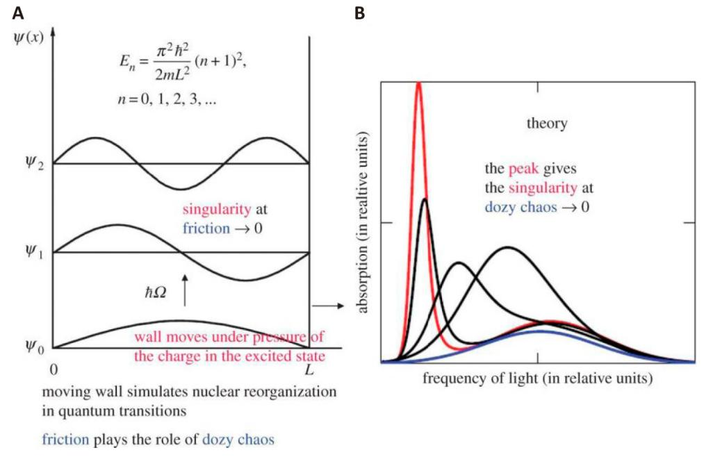
Figure 6. The Simplest Demonstration of Singularity in the Rate of Molecular “Quantum” Transitions[11,33-35]. A: The physical picture of quantum transitions in a potential box with a moving wall simulates the presence of a singularity in molecular “quantum” transitions when the wall moves without friction[11,33-35]. The case of a wall moving with friction corresponds to quantum–classical (dozy-chaos) mechanics[11,36-38,41], in which dozy chaos plays the role of friction. B: Egorov nano-resonance (Enr) depending on the dozy-chaos energy γ (Equations (29-31), (65-85))[11,33-35]. The optical absorption band with the most pronounced peak (J-band, red) corresponds to the smallest γ=0.2eV (θ0≡E⁄γ=5). The Gaussian-like band (blue) corresponds to the largest γ=3.3eV (θ0=0.3). The remaining parameters have the following numerical values: γ=0.25, 0.5, 1.0eV (black bands), m=m­e, where m­e is the electron mass; J1=5eV; formally J1-J2=0 for simplicity; E=1eV; corresponding LEnr=0.44 nm; ω=5×1013s-1; and T=300K. Reprinted (Adapted) with Permission from The Royal Society of Chemistry.

 

From the above it follows that the potential energy surfaces , being, as a rule, dynamic (adiabatic) invariants for the initial and final states of the electron‒nuclear system, are not dynamic invariants in the general case which includes a transient state. Therefore, the problem of dynamics for the transient state arises. Given the complexity of this problem as a whole, we solve the electron‒nuclear(‒vibrational) problem taking into account the dynamics of the transient state in the simplest case of “chemical transformations”, namely, in the case of elementary electron transfers in condensed matter. The comparative simplicity of this problem is related to the sufficiency of taking into account only the non-local phonons in the matter and the possibility of approximating the electron Green’s function by the propagator[11,37].

 

5 QCM OF ELEMENTARY ELECTRON TRANSFERS IN CONDENSED MEDIA IN BRIEF

The starting point in the construction of QCM of elementary electron transfers, or, according to Petrenko & Stein[18], Egorov’s theory (see above, Section 3.4), is the theory of multiphonon transitions[3,4]. The theory of multiphonon transitions was created in the late forties and early fifties by Huang & Rhys[106], Feynman[107], Lax[108], Krivoglaz & Pekar[109,110], and Kubo & Toyozawa[111], who used various mathematical methods to describe the electron-phonon interaction, from the method of generating polynomials to the density matrix method and methods of quantum field theory[3]. In practice, for further development of the theory, especially for creating the foundations of quantum–classical mechanics in the form of the theory of elementary electron-charge transfers in condensed matter, the method of generating polynomials of Krivoglaz & Pekar[109,110] turned out to be the most effective[11,18,20,37,38]. The method of generating polynomials originates from the Darwin–Fowler method in statistical physics[112] and takes into account only the main effect of electron-phonon interactions, namely, shifts of normal phonon coordinates during electron transitions. Effects of a higher order of smallness, such as the frequency effect, entanglement of normal phonon coordinates, etc., can be taken into account by other methods[3].

 

The simplest case of QCM – the case of elementary electron transfers in condensed matter[11] – is remarkable for the discovery of the Egorov nano-resonance[36-38]. The corresponding resonant transition is localized between the electron donor and acceptor separated by a distance of the order of a nanometer.

 

The electron-transfer Hamiltonian is as follows[3,11,16,17,36-38].

 

$$ H=-\frac{{\hslash }^{2}}{2m}{\Delta }_{\mathit{r}}+{V}_{1}\left(\mathit{r}\right)+{V}_{2}\left(\mathit{r}-\mathit{L}\right)+{\sum }_{\kappa }{V}_{\kappa }\left(\mathit{r}\right) {q}_{\kappa }+\frac{1}{2}{\sum }_{\kappa }\hslash {\omega }_{\kappa }\left({q}_{\kappa }^{2}-\frac{{\partial }^{2}}{\partial {q}_{\kappa }^{2}}\right)\left(43\right)$$

 

qκ and ωκ are the real normal phonon coordinates and frequencies (κ is the phonon index), V1(r) and V2(r-L) are the donor 1 and acceptor 2 potential wells of the electron (see also Section 3.4), and ∑κVκ(r) qκ is the electron‒phonon coupling.

 

The reorganization energy

 

$$ E=\frac{1}{2}{\sum }_{\kappa }\hslash {\omega }_{\kappa }{\stackrel{~}{q}}_{\kappa }^{2}\left(44\right)$$

 

where are the shifts of qκ.

 

An attempt to calculate the rates of “quantum” transitions taking into account the dynamics of the transient state using the Green’s function method with Hamiltonian (43) leads to a singular result[36-38].

 

This singularity is eliminated by replacing the infinitesimally small γ with a finite quantity[11,16,17,33-38] in the Green’s function.

 

$$ {G}_{H}\left(\mathit{r},{\mathit{r}}^{\text{'}};q,{q}^{\text{'}};{E}_{H}\right)={\sum }_{s}\frac{{\Psi }_{s}\left(\mathit{r},q\right) {\Psi }_{s}*\left({\mathit{r}}^{\text{'}},{q}^{\text{'}}\right)}{{E}_{H}-{E}_{s}-i\gamma }\left(45\right)$$

 

where Ψs(r,q) are the eigenfunctions of the Hamiltonian (43); (r,q) are all electronic and nuclear coordinates; Es are the eigenvalues of H, and EH is the total energy of the system. The aforementioned replacement of γ with a finite quantity in Equation (45), or in similar Green’s functions of more complex molecular and/or condensed matter systems, lies at the foundation of a new theory—dozy-chaos or quantum–classical mechanics (cf. Section 1)[11].

 

The dozy-chaos energy γ is a parameter that characterizes the measure of classicality and/or quantumness of a quantum-classical system. In the limit γ→0, the quantum-classical system becomes a singular quantum system (see below, Sections 6-8). At a qualitative level, the dozy-chaos energy γ can be imagined roughly as an imaginary part of some complex reorganization energy , in which the real part is the reorganization energy of nuclei E (see Equation (44))[35]:

 

$$ \stackrel{~}{E}=E+i\gamma $$

 

A significant milestone in the development of quantum–classical mechanics is the recent review by Egorov[11], where the mathematical apparatus of the new theory is presented in detail. Therefore, to study the mathematical apparatus of quantum–classical mechanics, we refer the reader to Egorov’s detailed discussion[11]. Here we will only outline the contours of the theory in broad strokes (for details, see Section replace 5 with 2.4 therein)[11].

 

The article by Egorov[11] formulated an adiabatic approximation in relation to elementary electron transfers in condensed matter and obtained the corresponding adiabatic wave functions of the system corresponding to the localization of the electron on the donor and/or on the acceptor. In relation to elementary electron transfers, the technique of modified Green’s functions has been formulated, on the basis of which the chaotic dynamics of the transient state is taken into account. The modification is expressed in replacing the infinitesimal imaginary addition iγ in the energy denominator of the complete Green’s function of the system with a finite value (see above). In theory, the smallness parameter

 

$$ \frac{\hslash \omega }{\gamma }\ll 1\left(46\right)$$

 

has been obtained, which ensures the convergence of the series of TDPT discussed in Section 4. Since the initial and final states are taken in the adiabatic approximation, the parameter from Equation (46) relates only to the transient state described by the formalism of modified Green’s functions.

 

An expression is obtained for the Green’s function of elementary electron transfers in condensed matter. The Green’s function is subsequently used to calculate the general expression for the rate constant of elementary electron photo-transfers using the generalized method of generating polynomials. This method, proposed by Egorov[37], generalizes the method of generating polynomials of Krivoglaz & Pekar[109,110]. The method of generating polynomials of Krivoglaz & Pekar is used for summation over all final phonon states of the system. The Egorov’s method allows summation not only over all final phonon states of the system, but also over all intermediate phonon states corresponding to the transient state of the quantum–classical system “electron + nuclear environment”. A general analytical expression for elementary electron transfers in condensed matter is obtained in the form of a double sum of a triple contour integral, which contains both the physical characteristics of the electron and the physical characteristics of the medium, and their interaction. The mathematical expression of the physical characteristics of the electron is the Green’s function of elementary electron transfers GE(ω1,L), which depends on the energy ω1 of intermediate phonon states. The mathematical expression of the physical characteristics of the medium is the product of two generating functions of three variables x, y, and z which are “linked” with the phonon arguments ω1 and ω1' of the intermediate states of two Green’s functions of elementary electron transfers GE(ω1, L) and GE*(ω1', L) via the aforementioned triple contour integral. The presence of both the Green’s function GE(ω1,L) and its complex conjugate GE*(ω1', L) corresponds to the presence of the squared modulus of the transition amplitude in the general result for transition rates in quantum mechanics. One variable z in the generating functions and corresponds to summation over all energies of final phonon states of the system, as in the standard theory of multiphonon transitions, and the other two variables x and y correspond to summation over all energies of intermediate phonon states.

 

The general expression for the optical absorption is as follows[11,37].

 

$$ K={c}_{12}^{2}{\sum }_{{\omega }_{1}=-\infty }^{\infty }{\sum }_{{\omega }_{1}^{\text{'}}=-\infty }^{\infty }{G}^{E}\left({\omega }_{1},L\right){G}^{E}*\left({\omega }_{1}^{\text{'}},L\right)$$

$$ \times \frac{1}{{\left(2\pi i\right)}^{3}}\oint \frac{dx}{{x}^{{\omega }_{1}+1}}\oint \frac{dy}{{y}^{{\omega }_{1}^{\text{'}}+1}}\oint \frac{dz}{{z}^{{\omega }_{12}+1}}Q\left({\stackrel{̄}{n}}_{1};x,y,z\right)S\left({\stackrel{̄}{n}}_{1};x,y,z\right)\left(47\right)$$

 

where

 

$$ {G}^{E}={G}^{E}\left(\alpha ,L\right)=\frac{1}{L}\left[\frac{\mathit{exp}\left(-\alpha L\right)+f\left(\alpha ,L\right)}{\left({\alpha }_{1}^{2}-{\alpha }^{2}\right){\left({\alpha }_{2}^{2}-{\alpha }^{2}\right)}^{2}}\right]\left(48\right)$$

 

$$ f\left(\alpha ,L\right)\equiv \left\{\left[1+\frac{\left({\alpha }_{2}^{2}-{\alpha }_{1}^{2}\right)L}{2{\alpha }_{2}}\right]\mathit{exp}\left(-{\alpha }_{2}L\right)-\mathit{exp}\left(-{\alpha }_{1}L\right)\right\}\frac{{\left({\alpha }_{2}^{2}-{\alpha }^{2}\right)}^{2}}{{\left({\alpha }_{2}^{2}-{\alpha }_{1}^{2}\right)}^{2}}$$

$$ -\left[\frac{L}{2{\alpha }_{2}}\mathit{exp}\left(-{\alpha }_{2}L\right)\right]\left({\alpha }_{2}^{2}-{\alpha }^{2}\right)-\mathit{exp}\left(-{\alpha }_{2}L\right)\left(49\right)$$

 

where the function α=α(ω1) is given as follows

 

$$ \alpha \equiv \alpha \left({\omega }_{1}\right)=\frac{{\left[2m\left({J}_{1}+\hslash {\omega }_{1}+i\gamma \right)\right]}^{\frac{1}{2}}}{\hslash }\left(50\right)$$

 

where, in turn,

 

$$ {{\omega }}_{1}\equiv {\sum }_{{\kappa }}{{\omega }}_{{\kappa }}\left({{n}}_{{\kappa }}-{{n}}_{{\kappa }1}\right)\left(51\right)$$

 

nκ are quantum numbers in the formula for the energy of a harmonic oscillator

 

$$ {\hslash }{{\omega }}_{{\kappa }}\left({{n}}_{{\kappa }}+\frac{1}{2}\right),{{n}}_{{\kappa }}=0,1,2,\dots .$$

 

In Equations (48) and (49)

 

$$ {\alpha }_{{1,2}}=\frac{{\left[2m\left({J}_{{1,2}}-E\right)\right]}^{1/2}}{\hslash }\left(52\right)$$

 

where J1 and J2 are the binding energies of the electron at the donor 1 and acceptor 2; E is the nuclear reorganization energy introduced in Equation (44). In Equation (47), c122 is a certain constant[11];

&nbsp;

$$ {\omega }_{12}\equiv {\sum }_{\kappa }{\omega }_{\kappa }\left({n}_{\kappa 2}-{n}_{\kappa 1}\right)\left(53\right)$$

 

And

 

$$ S\left({\stackrel{̄}{n}}_{1};x,y,z\right)=\mathit{exp}\left\{-{\sum }_{\kappa }{\stackrel{~}{q}}_{\kappa }^{2}\left(2{\stackrel{̄}{n}}_{\kappa 1}+1\right)+\frac{1}{2}{\sum }_{\kappa }{\stackrel{~}{q}}_{\kappa }^{2}\left[\left({\stackrel{̄}{n}}_{\kappa 1}+1\right)\left({x}^{{\omega }_{\kappa }}{y}^{{\omega }_{\kappa }}+1\right){z}^{{\omega }_{\kappa }}\right.\right.$$

$$ \left.\left.+{\stackrel{̄}{n}}_{\kappa 1}\left({x}^{-{\omega }_{\kappa }}{y}^{-{\omega }_{\kappa }}+1\right){z}^{-{\omega }_{k}}\right]\right\}\left(54\right)$$

 

$$ Q\left({\stackrel{̄}{n}}_{1};x,y,z\right)=\frac{1}{4}{\left\{{\sum }_{l}{\omega }_{l}{\stackrel{~}{q}}_{l}^{2}\left[1+\left({\stackrel{̄}{n}}_{l1}+1\right){\left(xyz\right)}^{{\omega }_{l}}-{\stackrel{̄}{n}}_{l1}{\left(xyz\right)}^{-{\omega }_{l}}\right]\right\}}^{2}$$

$$ +\frac{1}{2}{\sum }_{{l}}{{\omega }}_{{l}}^{2}{\stackrel{~}{{q}}}_{{l}}^{2}\left[\left({\stackrel{̄}{{n}}}_{{l}1}+1\right){\left({x}{y}{z}\right)}^{{{\omega }}_{{l}}}+{\stackrel{̄}{{n}}}_{{l}1}{\left({x}{y}{z}\right)}^{-{{\omega }}_{{l}}}\right]\left(55\right)$$

 

where is the Planck distribution function which arises due to averaging of the electron‒transfer rate constant over the equilibrium distribution of initial phonon states.

 

Next, in Equation (48), we expand the logarithm of the Green’s function of electron transfers GE(ω1,L)≡GE(J1+ℏω1;L) with respect to the intermediate levels of the electron energy ℏω1 in the vicinity of the donor level J1, where the overwhelming number of intermediate phonon states are concentrated[11,37]. In this expansion, restricting ourselves to the linear approximation, we obtain a double Laurent series, which, using Cauchy’s theorem

 

$$ f\left(z\right)={\sum }_{n=-\infty }^{\infty }{c}_{n}{\left(z-{z}_{0}\right)}^{n},{c}_{n}=\frac{1}{2\pi i}\oint \frac{f\left(\zeta \right)}{{\left(\zeta -{z}_{0}\right)}^{n+1}}d\zeta \left(56\right)$$

 

(the contour encircles the point z0, in the particular case z0=0), can be summed up accurately. Namely, we have

 

$$ {G}^{E}\left({J}_{1}+\hslash {\omega }_{1};L\right)\approx {G}^{E}\left({J}_{1};L\right)\mathit{exp}(-t{\omega }_{1}\left)\right(57)$$

 

$$ t=-{\left[\partial \mathit{ln}{G}^{E}\left({J}_{1}+\hslash {\omega }_{1};L\right)/\partial {\omega }_{1}\right]}_{{\omega }_{1}=0}\left(58\right)$$

 

Substituting the approximate expression (57) into the exact result (Equation (47)) and using the Cauchy theorem as applied to the Laurent series (Equation (56)), we get[11,37]

&nbsp;

$$ K={c}_{12}^{2}{\left|{G}^{E}\left({J}_{1};L\right)\right|}^{2}\times \frac{1}{2\pi i}$$

$$ \oint \frac{dz}{{z}^{{\omega }_{12}+1}}Q\left({\stackrel{̄}{n}}_{1};x={e}^{-t},y={e}^{-t},z\right)S\left({\stackrel{̄}{n}}_{1};x={e}^{-t},y={e}^{-t},z\right)\left(59\right)$$

 

Where e-t≡exp(-t). It goes without saying that the application of the linear approximation for ln[GE(J1+ℏω1;L)] (see Equation (57)) imposes restrictions on the parameters of the problem; however, it can be shown that these restrictions are not severe[11,37,113].

&nbsp;

Methods for calculating the contour integral in Equation (59) are similar to those applied in the standard theory of multiphonon transitions[3]. In Equation (59), the generating function (see Equation (54)) is exponential with respect to the variable z, while the generating function (see Equation (55)) is a power function in z. Therefore, in a large in modulus thermal effect ℏω12, when the phonon frequencies

 

$$ {\omega }_{\kappa ,l}<<\left|{\omega }_{12}\right|\left(60\right)$$

 

we can put ωl equal to zero in quantity , which appears in . (In particular, the condition of Equation (60) means that we neglect the well-known zero-phonon line here; see on zero-phonon lines[4,5,114].) Thus, Q is not now dependent on z, and in Equation (59) it can be brought outside the integral character in the point z=1[11,37]:

&nbsp;

$$ {K}={{c}}_{12}^{2}{\left|{{G}}^{{E}}\left({{J}}_{1};{L}\right)\right|}^{2}{Q}\left({\stackrel{̄}{{n}}}_{1};{x}={{e}}^{-{t}},{y}={{e}}^{-{t}},{z}=1\right)$$

$$ \times \frac{1}{2{\pi }{i}}\oint \frac{{d}{z}}{{{z}}^{{{\omega }}_{12}+1}}{S}\left({\stackrel{̄}{{n}}}_{1};{x}={{e}}^{-{t}},{y}={{e}}^{-{t}},{z}\right)\left(61\right)$$

 

In the framework of the Einstein model of vibrations of nuclei ωκ=constant≡ω, in Equiation (61) the contour integral is calculated exactly. In order to obtain the result, one can use, for example, the well-known expansion in a series[115]:

 

$$ \mathit{exp}\left(Az+\frac{B}{z}\right)={\sum }_{n=-\infty }^{\infty }{z}^{n}{\left(\frac{A}{B}\right)}^{\frac{n}{2}}{I}_{n}\left(2\sqrt{AB}\right)\left(62\right)$$

 

where In(...) is the modified Bessel function. Applying once again the Cauchy theorem with respect to the Laurent series (see Equation (56)), from Equation (61), taking Equation (62) into account, we get

 

$$ K={c}_{12}^{2}{\left|{G}^{E}\left({J}_{1};L\right)\right|}^{2}Q\left({\stackrel{̄}{n}}_{1};x={e}^{-t},y={e}^{-t},z=1\right)$$

$$ \times \mathit{exp}\left[-\frac{2E}{\hslash \omega }\text{coth }{\beta }_{T}+\left({\beta }_{T}-t\right)\frac{{\omega }_{12}}{\omega }\right] {I}_{\frac{{\omega }_{12}}{\omega }}\left(\frac{2E\text{ cosh }t}{\hslash \omega \text{ sinh }{\beta }_{T}}\right)\left(63\right)$$

 

where βT≡ℏω⁄2kBT, T is the absolute temperature. Further, using the well-known asymptotic formula[115,116]

 

$$ {I}_{v}\left(x\right)\approx \frac{1}{\sqrt{2\pi x}}\mathit{exp}\left(x-\frac{{v}^{2}}{2x}\right),x\gg 1,v\le x\left(64\right)$$

 

As a result, we have the optical absorption K, which is completely expressed in elementary functions[11,36-38] and presented in the next section.

 

6 RESULT FOR THE SHAPE OF THE OPTICAL ABSORPTION BAND. NANO-RESONANCE

When using the Einstein model ωκ=constant≡ω, the result for the optical absorption K=K(Ω) (Ω is the circular frequency of light) is given by the following equations[11,37,38]:

 

$$ K={K}_{0}\mathit{exp}W\left(65\right)$$

 

$$ W=\frac{1}{2}\mathit{ln}\left(\frac{\omega \tau \text{sinh}{\beta }_{T}}{4\pi \text{cosh}t}\right)-\frac{2}{\omega \tau }\left(\text{coth}{\beta }_{T}-\frac{\text{cosh}t}{\text{sinh}{\beta }_{T}}\right)$$

$$ +\left({\beta }_{T}-t\right)\frac{1}{\omega \tau \Theta }-\frac{\text{sinh}{\beta }_{T}}{4\omega \tau {\Theta }^{2}\text{cosh}t}\left(66\right)$$

 

$$ 1\ll \frac{1}{\omega \tau \Theta }\le \frac{2\text{cosh}t}{\omega \tau \text{sinh}{\beta }_{T}}\left(67\right)$$

 

$$ t=\frac{\omega {\tau }_{e}}{\theta }\left[\frac{AC+BD}{{A}^{2}+{B}^{2}}+\frac{2\Theta \left(\Theta -1\right)}{{\left(\Theta -1\right)}^{2}+{\left(\Theta /{\theta }_{0}\right)}^{2}}+\frac{{{\theta }_{0}}^{2}}{{{\theta }_{0}}^{2}+1}\right]\left(68\right)$$

 

$$ \left|{\theta }_{0}\right|\gg \frac{E}{2{J}_{1}}\left(69\right)$$

 

$$ \theta \equiv \frac{{\tau }_{e}}{\tau }=\frac{LE}{\hslash \sqrt{2{J}_{1}/m}},\Theta \equiv \frac{{\tau }^{\text{'}}}{\tau }=\frac{E}{\Delta },{\theta }_{0}\equiv \frac{{\tau }_{0}}{\tau }=\frac{E}{\gamma }\left(70\right)$$

 

$$ {\tau }_{e}=\frac{L}{\sqrt{2{J}_{1}/m}},\tau =\frac{\hslash }{E},{\tau }^{\text{'}}=\frac{\hslash }{\Delta },{\tau }_{0}=\frac{\hslash }{\gamma }\left(71\right)$$

 

Here, we use the notation

 

$$ A=\mathit{cos}\left(\frac{\theta }{{\theta }_{0}}\right)+\Lambda +{\left(\frac{1}{{\theta }_{0}}\right)}^{2}{\rm N}\left(72\right)$$

 

$$ B=\mathit{sin}\left(\frac{\theta }{{\theta }_{0}}\right)+\frac{1}{{\theta }_{0}}{\rm M}\left(73\right)$$

 

$$ C=\theta \left[\mathit{cos}\left(\frac{\theta }{{\theta }_{0}}\right)-\frac{1-{\xi }^{2}}{2{\theta }_{0}}\mathit{sin}\left(\frac{\theta }{{\theta }_{0}}\right)\right]+{\rm M}\left(74\right)$$

 

$$ D=\theta  \left[\mathit{sin}\left(\frac{\theta }{{\theta }_{0}}\right)+\frac{1-{\xi }^{2}}{2{\theta }_{0}}\mathit{cos}\left(\frac{\theta }{{\theta }_{0}}\right)\right]-\frac{2}{{\theta }_{0}}{\rm N}\left(75\right)$$

 

And

 

$$ \xi \equiv {\left(1-\frac{E}{{J}_{1}}\right)}^{1/2}\left({J}_{1}>E{b}{y}{d}{e}{f}{i}{n}{i}{t}{i}{o}{n}\right)\left(76\right)$$

 

and where we finally have

 

$$ \Lambda =-{\left(\Theta -1\right)}^{2}{\rm E}+\left[\frac{\left(\Theta -1\right)\theta }{\rho }+\Theta \left(\Theta -2\right)\right]{{\rm E}}^{\frac{1-\rho }{1-\xi }}\left(77\right)$$

 

$$ {\rm M}=2\Theta \left(\Theta -1\right){\rm E}-\left[\frac{\left(2\Theta -1\right)\theta }{\rho }+2\Theta \left(\Theta -1\right)\right]{{\rm E}}^{\frac{1-\rho }{1-\xi }}\left(78\right)$$

 

$$ {\rm N}=\Theta \left[\Theta {\rm E}-\left(\frac{\theta }{\rho }+\Theta \right){{\rm E}}^{\frac{1-\rho }{1-\xi }}\right]\left(79\right)$$

 

$$ {\rm E}\equiv \mathit{exp}\left(\frac{2\theta }{1+\xi }\right),\rho \equiv \sqrt{{\xi }^{ 2}+\frac{1-{\xi }^{ 2}}{\Theta }}\left(80\right)$$

 

The factor K0 becomes

 

$$ {K}_{0}={K}_{0}^{e}{K}_{0}^{p}\left(81\right)$$

 

where

 

$$ {K}_{0}^{e}=\frac{2{\tau }^{3}{J}_{1}}{m}\frac{\left({A}^{2}+{B}^{2}\right){\rho }^{3}{\Theta }^{4}\xi }{{\theta }^{2}{\left[{\left(\Theta -1\right)}^{2}+{\left(\frac{\Theta }{{\theta }_{0}}\right)}^{2}\right]}^{2}\left[1+{\left(\frac{1}{{\theta }_{0}}\right)}^{2}\right]}\cdot \eta \left(82\right)$$

 

And

 

$$ \eta \equiv \mathit{exp}\left(-\frac{4\theta }{1-{\xi }^{2}}\right)\left(83\right)$$

 

and

 

$$ {K}_{0}^{p}=\frac{1}{\omega \tau }{\left[1+\frac{\text{sinh}\left({\beta }_{T}-2t\right)}{\text{sinh }{\beta }_{T}}\right]}^{2}+\frac{\text{cosh}\left({\beta }_{T}-2t\right)}{\text{sinh }{\beta }_{T}}\left(84\right)$$

 

In Equations (70) and (71), Δ≡ℏω12 is the thermal energy included in the energy conservation law:

 

$$ \hslash \Omega ={J}_{1}-{J}_{2}+\Delta \left(85\right)$$

 

where J1 and J2 are the binding energies of the electron at the donor 1 and acceptor 2 introduced in Section 5; E is the nuclear reorganization energy (Equation (44)); γ is the dozy-chaos energy[16,17]; L is the donor–acceptor distance (see above, Sections 3.4 and 5) or the length of the polymethine chain—the main optical chromophore of polymethine dyes (see below, Section 11)[11,16,17,33-35,36-38,49,60,117]; m is the effective mass of the electron (Sections 3.4 and 5). The time scales given by Equation (71) are discussed in Egorov[11,17,34,38,60], where

 

$$ {\tau }_{e}=\frac{L}{\sqrt{2{J}_{1}/m}}$$

 

and

 

$$ \tau =\frac{\hslash }{E}$$

 

are included in the Egorov nano-resonance as follows

 

$$ {\left(2{\tau }_{e}\right)}^{-1}={\tau }^{-1}$$

 

(see above, Section 3.4, Equations (29-31)).

 

The extinction coefficient ε measured experimentally is related to the optical absorption K by the equation[3]:

 

$$ {\epsilon }=\frac{4{{\pi }}^{2}{{q}}^{2}{{N}}_{{A}}{\Omega }}{3{\hslash }{c}{{n}}_{\text{ref}}}{K}\left(86\right)$$

 

where q is the electron charge transferred in a quantum–classical transition, NA is the Avogadro constant, c is the speed of light in vacuum, and nref is the refractive index.

The physical meaning of all quantities included in Equations (65-85), as well as the dynamics of the formation of the shape of optical bands, are discussed by Egorov[11].

 

The quantity K=K(Θ,θ0) (Equation (65)) and the corresponding optical extinction (Equation (86)) have a singularity at the point (Θ=1,θ0=∞) or(Δ=E,γ=0). The nature of this singularity is determined by singularities of the functions t=t(Θ,θ0) in Equation (68) and K0e=K0e(Θ,θ0) in Equation (82). The singularity in the function K0e=K0e(Θ,θ0) is removable[11,34,37]. In the function t=t(Θ,θ0), the singularity at the point (Θ=1,θ0=∞) is non-removable. The behavior of the function t=t(Θ,θ0) in the vicinity of the singular point is illustrated in Egorov’s studies[11,34,37].

 

Below (Sections 7-9) it is shown that the result of Egorov’s theory on the shape of the optical band in the case of strong dozy chaos coincides with the corresponding result on the shape of the optical band obtained in quantum mechanics using the Franck–Condon principle (Figures (7) and (8)).

 

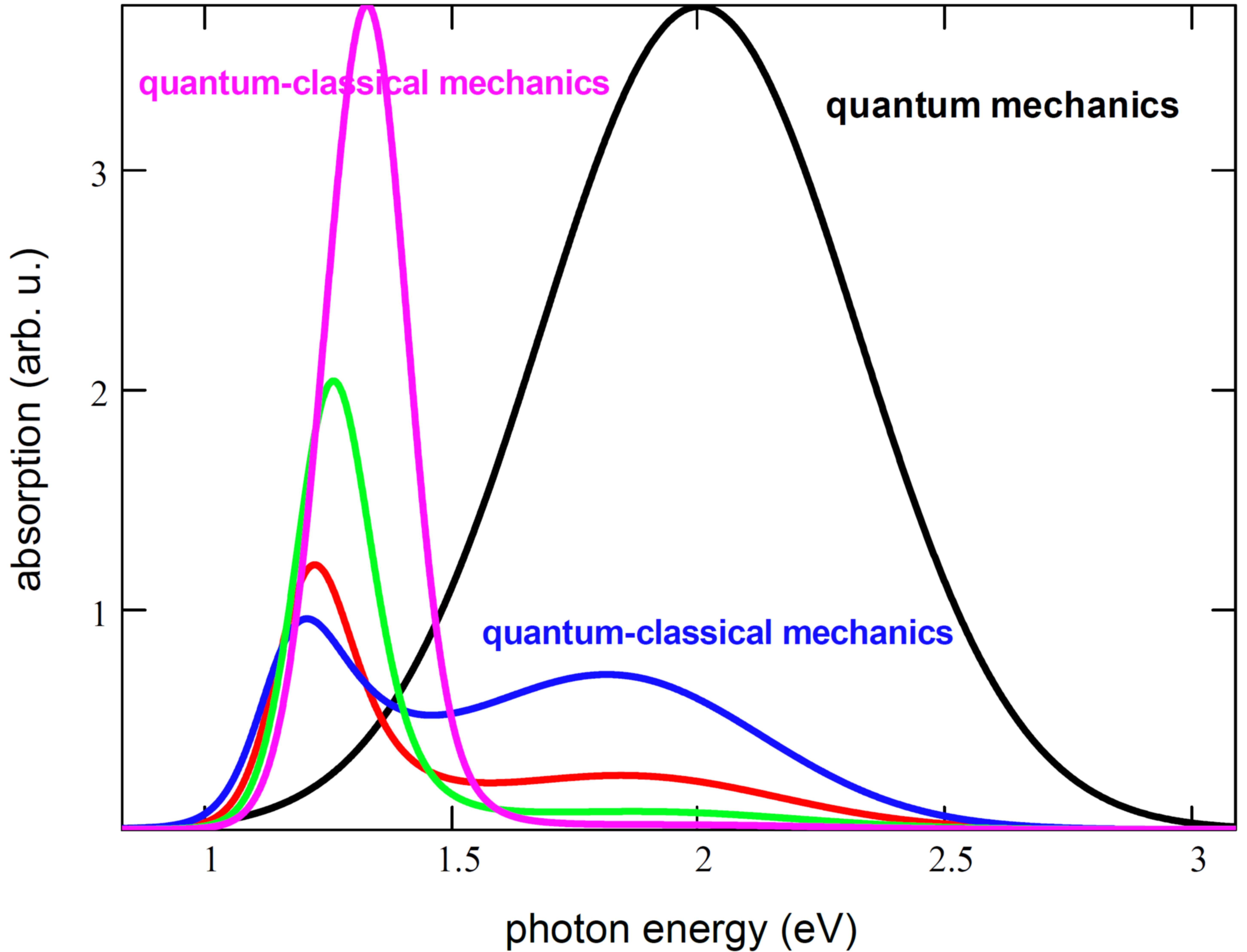
Figure 7. Gaussization of the Optical Band Shape in QCM with Shortening of the Transition Length L. QCM: Transformation of the theoretical absorption spectra of a model polymethine dye witha change in the length of QCT (different lengths of polymethine chains) L[47]. Optical bands are calculated from Equations (65-85) (η=1 in Equations (82) and (83)[16,17, 33-38]). The following numerical values of the parameters are used: m=m­e, where m­e is the electron mass; nref=1.33; ω=5×1013 s-1; J1=5 eV; J1-J2=0.5eV; E=1eV; γ=0.34eV; and T=298K[15,19]. In this figure, for simplicity, the energy gap J1-J2≡0. Extent of the quantum–classical transition L=1.4 L0 (blue), L0 (red), 0.7 L0 (green), 0.45 L0 (magic), where L0≡LEnr=0.384nm[15,19]. Quantum mechanics: Gaussian absorption spectrum (black) given by the standard theory (Equation (87), where E=1eV and T=298K are the same as in the case of quantum–classical mechanics)[47]. Reprinted (Adapted) from Ref.[47] with Permission from CC BY.

 

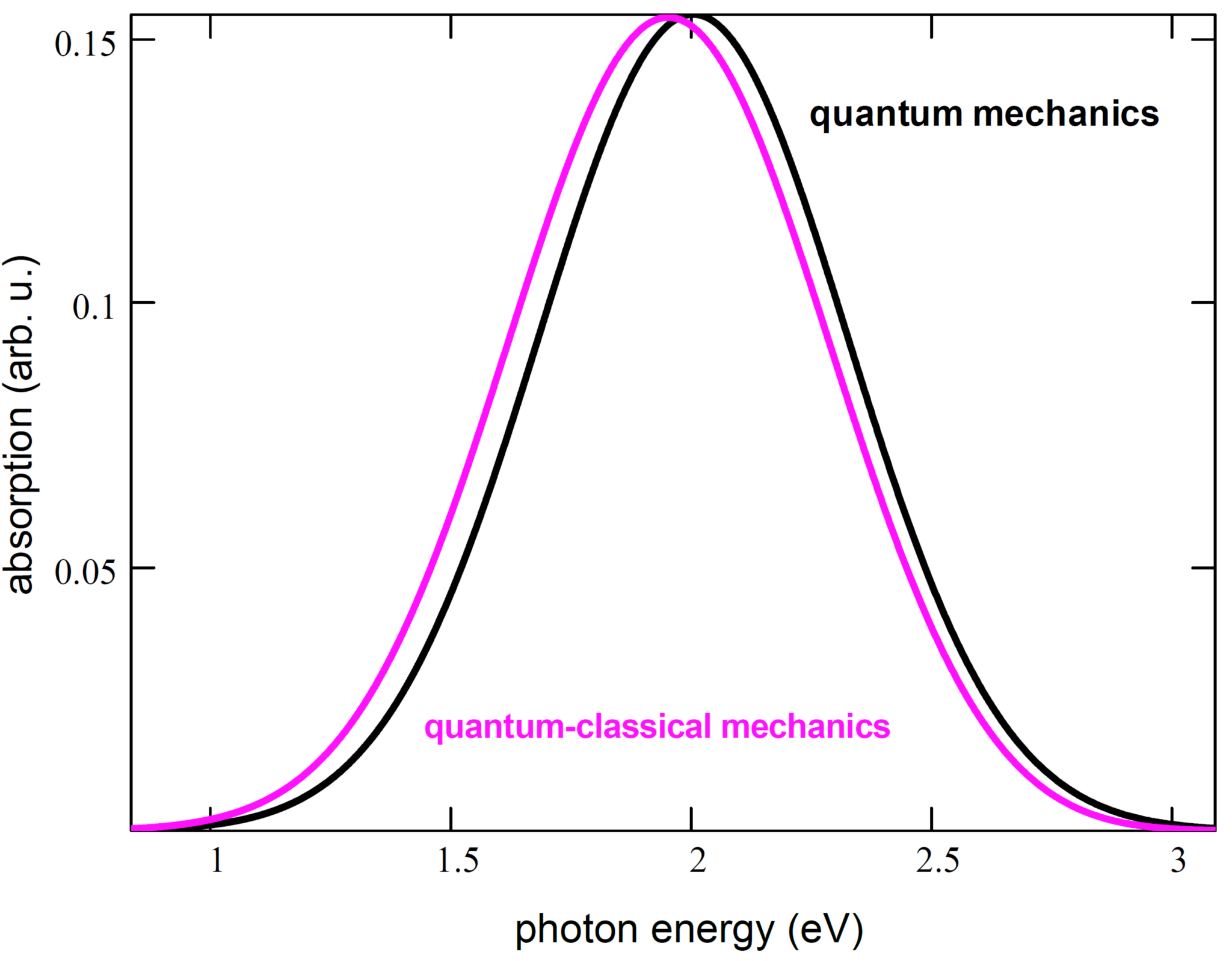
Figure 8. The Effect of the Coincidence of the Shape of the Optical Band in QCM with the Gaussian Shape of the Band in QM with a Shortening of the Transition Length L and a Moderate Increase in the Dozy-Chaos Energy γ. Illustration of the coincidence of the position and shape of optical bands in the case of electron-vibrational transitions of short extent L=0.45 L0 (magic curve), where the extension L0≡LEnr=0.384nm corresponds to Egorov’s nano-resonance, and/or strong dozy chaos (γ=3eV) in QCM and in the case of electron-vibrational transitions in the Franck–Condon picture in quantum mechanics (black curve). Increasing the γ parameter from 0.34eV (Figure 7) to 3eV. All other parameters are the same as in Figure 7[47]. Reprinted (Adapted) from Ref.[47] with Permission from CC BY.

 

7 PASSAGE FROM THE RESULT OF QCM TO THE RESULT OF STANDARD THEORY BASED ON QM

Just as there is no strict limit transition from quantum mechanics to classical mechanics, there is no strict limit transition from quantum–classical mechanics to quantum mechanics. The standard result in the theory of multiphonon transitions[3] is obtained from Equations (65-85) by γ→∞ (θ0→0 according to Equation (70)) in Equation (68) for t and by γ→0 (θ0→∞) in Equation (82) for K0e[11,37] :

 

$$ K=\frac{{a}^{2}\hslash }{\sqrt{4\pi {\lambda }_{r}{k}_{B}T}}{e}{x}{p}\left(-\frac{2L}{a}\right){e}{x}{p}\left[-\frac{{\left(∆-{\lambda }_{r}\right)}^{2}}{4{\lambda }_{r}{k}_{B}T}\right]\left(87\right)$$

 

where and λr≡2E. The Gaussian formula (the Marcus formula, see below)

 

$$ K=K\left(\Delta \right)\propto \mathit{exp}\left[-\frac{{\left(\Delta -{\lambda }_{r}\right)}^{2}}{4{\lambda }_{r}{k}_{B}T}\right]$$

 

is the well-known simplest result in the theory of multiphonon transitions for kB T>ℏω⁄2[3,4]. It is associated with the works of Marcus on his electron‒transfer model[118-120], and with the previous works by Huang & Rhys[106], Pekar[116,121,122], Lax[108], Krivoglaz & Pekar[109], and Krivoglaz[110]. Usually, the aforementioned Gaussian formula is called the Marcus formula, and the energy λr is called the Marcus reorganization energy (cf. Section 3.4). Equations (65-85) properly take into account the dynamics of the transient state, their chaotic and regular parts. On the contrary, in Equation (87) and the Marcus formula, the dynamics of the transient state are completely ignored.

 

It can be seen that the result of QCM (Equations (65-85)) does not transform into any result of quantum mechanics in any of the limiting cases of γ, zero or infinity. With γ→0, we get infinity for the transition rate, and with γ→∞, we get zero for it. This situation is easy to understand from a qualitative examination of quantum–classical transitions in a potential box with a movable wall, the movement of which simulates the reorganization of the positions of the nuclei in space during electronic transitions, see Figure 6A; the graphs in Figure 6B (Equations (65-85)) explain this situation as well[11,16,17,34].

 

8 THE SIMPLEST PHYSICS OF QCT. NANO-RESONANCE: L-PEAK AND D-BAND

In Figure 6B (Section 4), the shift of the peak of the optical band to the red side, its narrowing and increase in intensity with decreasing γ is explained by a decrease in friction at the base of the moving wall (see Figure 6A): greater mobility of the wall leads to a greater decrease in the effective gap between the ground and excited electronic energy levels and more a high degree of organization of the QCT. In Egorov nano-resonance, the width and intensity of the optical band peak, as well as its red position on the frequency axis, are very sensitive to changes in γ, while the high-frequency wing of the optical band weakly depends on γ (Figure 6B, caption). Therefore, in Petrenko et al.[20] and Egorov[37], the peak of Egorov’s nano-resonance is called the L-band (living band) or L-peak, and its wing is called the D-band (dead band).

 

The absence of a rigorous transition from QCM to quantum mechanics (Section 7) indicates the fundamental novelty of QCM, which in principle cannot be reduced to quantum mechanics[15].

 

The simplest physics of quantum–classical transitions is discussed in more detail in the next section.

 

9 RELATIVE CHARACTER OF THE INTENSITY OF DOZY CHAOS

The intensity of dozy chaos, characterized by the value γ, is relative, that is, the same intensity of chaos is small for transitions with a large extent L, and vice versa, large for transitions with a small extent L[47]. This fact is illustrated in Figure 7 (Section 6). At a sufficiently small value of γ, corresponding to the weak intensity of dozy chaos (γ<<E, see Sections 1 and 3.4), a decrease in the transition length L turns the complex optical absorption curve (blue) into a Gaussian curve (magic), which, as we saw above (Sections 6 and 7), corresponds to the strong intensity of dozy chaos (γ≅E or γ>>E).

 

An explanation for the shift of the Gaussian band (magic) to the red region and its narrowing in relation to the Gaussian band (black) from quantum mechanics can be given by considering a potential box with a moving wall (Figure 6A). A moving wall models nuclear reorganization in QCM and has a much less “mass” compared to the “mass” of a stationary wall in quantum mechanics, where “mass” is related to the value of the reorganization energy E in the same way that friction at the base of a wall is related to the value of the dozy-chaos energy γ, as discussed above (see Section 4, caption to Figure 6; and Section 8). This analogy in explanations using the “mass” of the moving wall of a potential box and friction at its base correlates with a rough representation of the dozy-chaos energy γ at a qualitative level, which, as noted in Section 5, can be considered as the imaginary part of some complex reorganization energy , in which the real part is the reorganization energy of nuclei E[35]. More detailed explanations are given in Egorov’s studies[15,19,47].

 

Thus, from Figure 7 it follows that both the dozy-chaos energy γ and the extent of quantum–classical transitions L are a measure of dozy chaos. In other words, the intensity of dozy chaos is relative in nature, since in addition to the energy γ, it is also determined by the extent L.

 

An increase in the dozy-chaos energy γ from 0.34eV to 3eV for the optical band corresponding to the shortest length L=0.45 L0 (magic) and corresponding to quantum–classical mechanics in Figure 7, leads to the coincidence of the width and position of both Gaussian curves corresponding to quantum–classical mechanics and quantum mechanics (Figure 8). With this we complete the illustration of quantitative confirmation of the illusory nature of the Franck‒Condon principle (Section 2) using the example of Egorov’s theory[47]. However, in conclusion, we note that the fact that the results of quantum–classical mechanics in the case of short transitions and/or strong dozy chaos coincide with the corresponding results of standard quantum mechanics is general. In other words, this applies not only to Egorov’s theory, but also to all QCM as a whole, which has yet to be created in the future. This conclusion seems obvious if we take into account that above we made a “long-limit transition” from a very well-organized dynamical system containing a unique result in a narrow and intense J-band of J-aggregates, to a completely unorganized system. Whereas such a “short transition to the limit” from a poorly organized dynamical system, represented in standard spectroscopy by relatively small molecules, would occur in an even more obvious way with a decrease in some effective L and/or an increase in γ.

 

10 APPLICABILITY OF QCM TO BOTH SOLIDS AND LIQUIDS

In Egorov’s theory[11,37], as in the standard theory of multiphonon processes[3,121,122], it is assumed that atoms oscillate around certain equilibrium positions, which do not necessarily form a regular periodic configuration. Therefore, in both of these theories, at sufficiently short times, the liquid does not differ from a solid body. However, these “short” times turn out to be quite long, if we take into account that the times of elementary electron transfers τtr≅τ=ℏ⁄E are significantly less than the times of mixing of liquid τT≅ℏ⁄kBT due to strong statistical fluctuations (kBT<<E, since at room temperature kBT=1⁄40eV and E=(1÷0.1)eV)[11]. This picture is confirmed by the successful explanation of the optical spectra of polymethine dyes and their aggregates in liquid solutions based on Egorov’s theory (see below).

 

11 SIMULATION OF EXTENDED TRANSITIONS IN CHROMOPHORES OF POLYMETHINE DYES ACCORDING TO EGOROV’S THEORY

The main optical chromophore of polymethine dyes is a polymethine chain with a length of the order of a nanometer or more. In the polymethine chain, the charge on neighboring carbon atoms has a different sign (Figure 9). Upon optical excitation, this alternating charge distribution is alternately redistributed, which makes it possible to consider the charge redistribution along the chain as a sequence of several charge transfer acts between neighboring carbon atoms, following each other. Due to the small distances between carbon atoms, this process can be represented as a single elementary transfer of electronic charge along the entire chain of length L with a tunneling factor η in Egorov’s theory less than or on the order of unity (Section 6, Equations (82) and (83), η≤1)[16,17,33-38]. For sufficiently long polymethine chains, the number of vibrational modes of the nuclei of the medium that effectively interact with the electronic transition significantly exceeds the number of intramolecular vibrational modes that effectively interact with it. This circumstance allows us to neglect local phonons and limit ourselves to taking into account only nonlocal phonons, which significantly simplifies the calculation problem[3,11,37]. An experimental consequence of such a dominant role of nonlocal phonons is the Egorov nano-resonance (Equation (29)), which is observed both for J-aggregates (see below, Section 12, Figure 11A, 11B and 12) and for monomers of polymethine dyes (Figure 10A).

 

Figure 9. The Ground State of a Quasilinear Polymethine Chain with Alternating Positive (1) and Negative (2) Charges on Carbon Atoms[35,92,93]. The chain length L is determined by the distance between nitrogen atoms (N). Reprinted (Adapted) with Permission from The Royal Society of Chemistry.

 

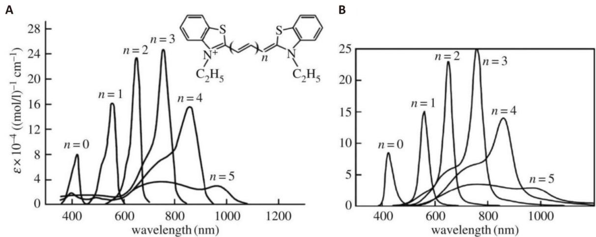
Figure 10. Transformation of the Optical Absorption Band of a Thiacarbocyanine Dye in Methanol with Varying Length of the Polymethine Chain L=2(n+2)d, where d are Certain Roughly Equal Bond Lengths in the Chain. Absorption bands are computed by Equations (65-86) with η≤1 instead of the Gamow exponent exp(-4θ⁄(1-ξ2)) (Equations (82) and (83))[34,35]; the wavelength λ=2πc⁄Ωnref; (A) experiment[21,123], (B) theory[11,38]. The chain length L for n=3 corresponds to Egorov’s nano-resonance (L=1.4nm). We used the “dye + environment” system parameters[38] q=e, where e is the electron charge, m=me, ω=5×1013s-1, d=0.14nm, nref=1.33; for n=0,1,2,3,4,5 we respectively have J1=(5.63, 5.40, 4.25, 3.90, 3.74, 3.40)eV, J1-J2=(1.71, 1.31, 1.11, 0.90, 0.74, 0.40)eV, E=(0.245, 0.248, 0.256, 0.275, 0.297, 0.496)eV, and γ=(0.402, 0.205, 0.139, 0.120, 0.129, 0.131) eV. For short chains (n=0,1,2,3), tunnel effects can be neglected (η=1). For long chains (n=4,5), although the tunnel effects are small, they must be taken into account (η=0.55, 0.1). T=298K. Reprinted (Adapted) with Permission from The Royal Society of Chemistry.

 

Figure 10 shows the change in the shape and intensity of the optical absorption band of a thiacarbocyanine dye in methanol with varying length of the polymethine chain L. The band with n=3 and/or L=1.4nm corresponds to the Egorov nano-resonance.

 

12 EXPLANATION OF THE J-BAND OF J-AGGREGATES BY NANO-RESONANCE. M–J CONCENTRATION EQUILIBRIA

A classic example of the formation of J-aggregates of polymethine dyes is the well-known Herz experiment[21,22] on the aggregation of benzimidazolocarbocyanine with increasing its concentration in an aqueous solution (see Figures 11A and 11B).

 

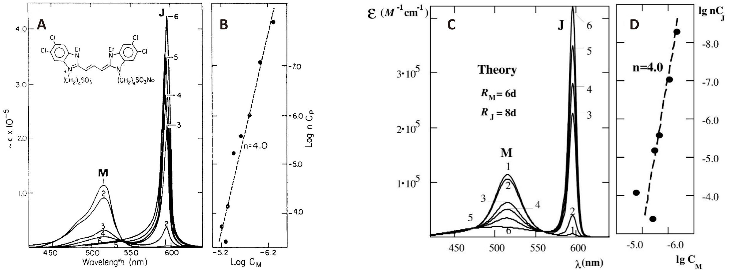
Figure 11. Formation of J-aggregates from Polymethine Dyes in an Aqueous Solution. (A,B) Experiment[21,22], (C, D) Theory[36,37]. At the (A and B): Concentration equilibria of monomers (M) of benzimidazolocarbocyanine and their J-aggregates (J) in an aqueous solution of NaOH (0.001mol l-1) at 25°C, and corresponding experimental data on optical absorption[21,22]. (A) Concentration of the dye is equal to 0.5 (1), 1.0 (2), 5.0 (3), 10 (4), 100 (5), and 400 (6) micromole/liter. (B) Finding the number of molecules n in the optical J-chromophore (see Figure 12) from the law of mass action for the dye concentrations (CM and CP) indicated above. At the (C and D): Fitting the theoretical result to the experimental data on the shape of the optical absorption bands given at the (A and B)[36-38]. (A) M- and J-bands are computed from Equations (65-86), where η=1. Percentage of dye in J-aggregates in solution with increasing dye concentration: 1% (1), 9% (2), 53% (3), 66% (4), 82% (5), and 99% (6). (B) Finding the number of molecules n in the optical J-chromophore from the law of mass action for the concentrations of monomers (CM) and J-aggregates (CJ), which are obtained from the absolute concentrations of the dye in the experiment (see the caption at the (A and B)) and the relative concentrations derived from our theoretical fitting (see above; n=4, cf. (B) at the (A and B)). The parameters used in Equations (65-86) for the “J-aggregate + environment” and “monomer + environment” systems are mJ=0.86me and mM=0.97me, ω=5×1013 s-1, d=0.14nm, nrefr=1.33; J1J=J1M=5eV, J1J-J2J=1.11eV and J1M-J2M=1.37eV, EJ=0.420eV and EM=0.315eV, γJ=0.067eV and γM=0.231eV; the total charges transferred along chromophores LJ≡RJ=8d =1.12nm and LM≡RM=6d=0.84nm of J-aggregate and monomer (Figure 12) are and , where permittivity εd=2.5 (contribution from σ-electrons and the solvent)[91]. Reprinted (Adapted) from Ref.[36] with Permission from Elsevier B.V.

 

Using the law of mass action, Herz showed that the optical chromophore of a J-aggregate consists of four dye molecules, which, according to Hans Kuhn[91], form a brickwork-like structure[22].

&nbsp;

The scheme for the formation of an optical J-chromophore from four dye monomers with a brickwork-like structure and the scheme for the formation of the entire J-aggregate, which has the form of a long thin rod, are shown in Figure 12[16,17,33,34,36-38].

 

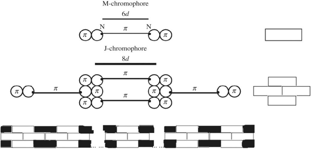
Figure 12. A Brickwork-like Structure of J-chromophore of Four Molecules and J-aggregate (bottom)[21,22,34,91]. The π-electron system of the polymethine chain stacks with the π-electron system of the benzene rings of two neighboring molecules (d is some unit bond length). The fourth molecule, fixing the brickwork, is assumed to be “neutral” in relation to the π -stacking in the other three molecules, and it acts only as a stabilizer of the J-chromophore structure[16,17,33,34,36-38]. Reprinted (Adapted) from Ref.[34] with Permission from CC BY.

 

The results of fitting the theoretical band shape (Equations (65-86)) to the Herz experimental data[21,22] (Figure 11A and 11B) are presented in Figure 11C and 11D[36,37].

 

The physical mechanism leading to the enhancement of the electronic transition in the Egorov nano-resonance is the stimulation of the electronic transition by the movement of nuclear reorganization of the medium under conditions of weak dozy chaos[15-17,34,36-38,49]. Compared to nano-resonance in monomers M (see Figure 10), a significant increase in nano-resonance in J-aggregates (Figure 11) is associated with the transition from the one-dimensional geometry of the optical M-chromophore to the two-dimensional geometry of the J-chromophore due to the stacking of the π-electronic structure of the quasi-one-dimensional polymethine chain of one molecule with π-electronic structures of flat benzene rings of two neighboring molecules (Figure 12), which leads to a significant increase in the interaction of the electronic transition with the surrounding nuclei and an increase in nano-resonance[15-17,33,34,36-38,49].

 

Note that the idea of π-stacking is widely used in the construction of various systems of organic molecules[124]. In 2001, Egorov applied the idea of π-stacking to explain the structure of J-aggregates[36,37]. The nature of π-interactions was first investigated by Hunter & Sanders[125]. The nature of π-stacking is being intensively studied using advanced quantum chemistry techniques[126-131].

 

We also note that shown in Figure 12 the structure of J-aggregates in the form of long thin rods minimizes the influence of parasitic excitonic effects between J-chromophores[16,17,36-38].

 

13 NANO-RESONANCE DEPENDING ON SOLVENT

Egorov’s nano-resonance (see Section 3.4, Equations (29-31); formerly “transferon resonance”[38]) for polymethine dyes in monomeric (not J-aggregated) form was first demonstrated in 2002 using the thiapolymethine cyanine series in solvent methanol, in which the length of the polymethine chain varies (Figure 10)[16,17,38]. Equations (29-31) in addition to the chain length L include the solvent reorganization energy E, the value of which directly depends on the polarity of the solvent. Therefore, it is of interest to study the dependence of the nano-resonance position on the polarity of the solvent. Figure 13 shows the change in the set of band shapes in Figure 10 with decreasing reorganization energy E[34]. It can be seen that the use of a solvent with lower polarity results in changing the sign of the relative intensity of the bands for the chain lengths n=2 and n=4, which are closest to the resonance band (n=3). This effect was first explained by Petrenko & Stein[20], using the corresponding experimental data for dyes from Kachkovski et al.[132] (see Scheme 1), where: (i) nano-resonance in a dye series (thiacyanines) is at n=3 [compare Figures 10 and 13A (methanol; n=2 and n=4) and Figure 14 (dichloromethane; labels 2 and 4)], and (ii) nano-resonance in a dye series (thiapyrylocyanines) is at n=2 [compare Figure 15 (dimethylsulphoxide; labels 2 and 4) and Figure 16 (dichloromethane; labels 2 and 4)].

 

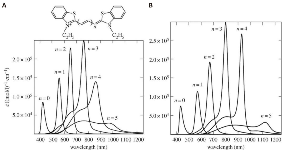
Figure 13. Theoretical Dependence of Optical Absorption of a Thiapolymethinecyanine Dye on the Polymethine Chain Length 2(n+2)d, where d are Certain Roughly Equal Bond Lengths in the Chain[38]. (A) the results are the same as in Figure 10B. (B) EB=0.8E and γB=(0.402, 0.205 X 1.2, 0.139 X 1.2, 0.120 /1.1, 0.129 /1.8, 0.131/1.5), the other parameters are the same as in Figure 10B[34]. Reprinted (Adapted) from Ref.[34] with Permission from CC BY.

 

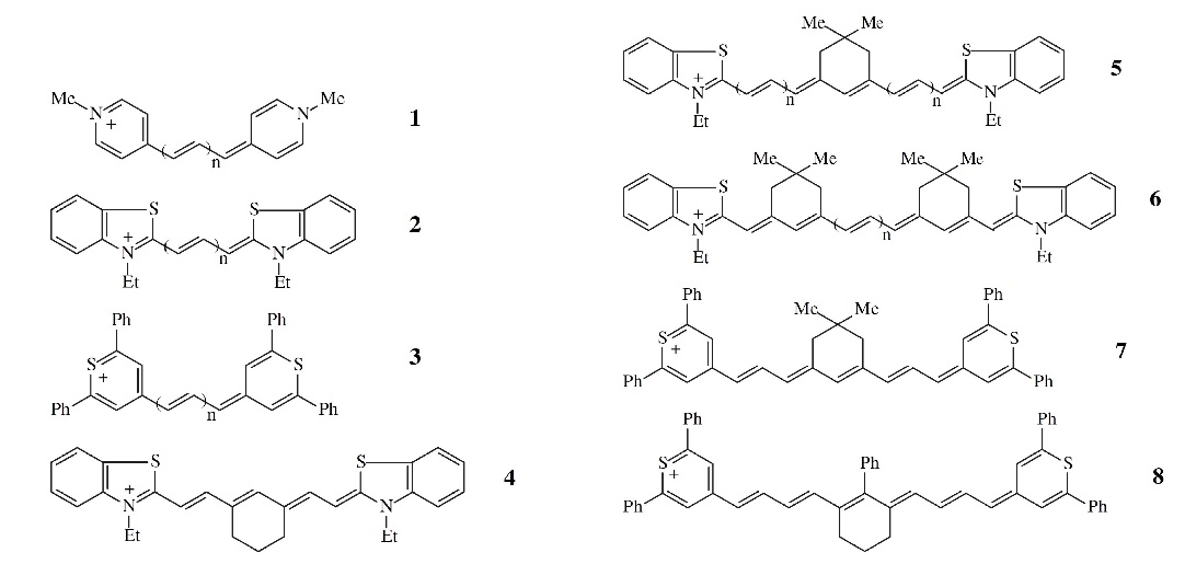
Figure 1Scheme 1. The Polymethine Dye Ions Studied in Kachkovski et al[132].

 

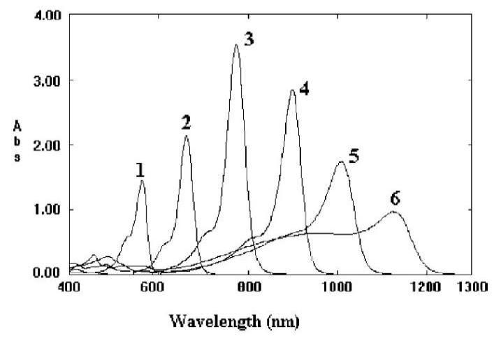
Figure 14. Absorption Spectra of Thiacyanines in Dichloromethane (10–5mol/L). 1, dye 2 (n=1) ; 2, dye 2 (n=2); 3, dye 2 (n=3); 4, dye 5 (n=1); 5, dye 7 (n=1); 6, dye 6 (n=2) (see Scheme 1). Reprinted (Adapted) from Ref.[132] with Permission from Elsevier B.V.

 

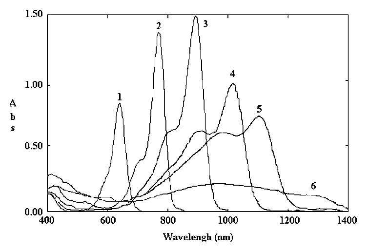
Figure 15. Absorption Spectra of Thiapyrylocyanines in Dimethylsulphoxide (8×10–6mol/L). 1, dye 3 (n=0); 2, dye 3 (n=1); 3, dye 3 (n=2); 4, dye 3 (n=3); 5, dye 7; 6, dye 8 (see Scheme 1). Reprinted (Adapted) from Ref.[132] with Permission from Elsevier B.V.

 

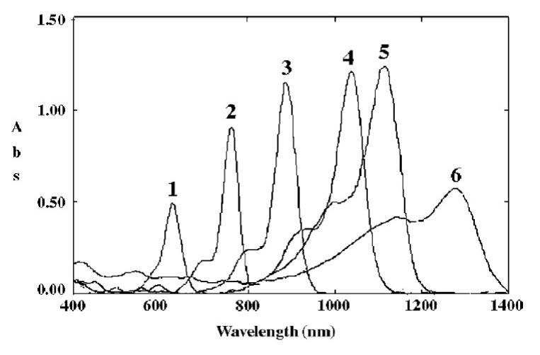
Figure 16. Absorption Spectra of Thiapyrylocyanines in Dichloromethane (4×10–6mol/L). 1, dye 3 (n=0) ; 2, dye 3 (n=1); 3, dye 3 (n=2); 4, dye 3 (n=3); 5, dye 7; 6, dye 8 (see Scheme 1). Reprinted (Adapted) from Ref.[132] with Permission from Elsevier B.V.

 

In conclusion, we note that the explanation of the experimental data in Kachkovski et al.[132] on an increase in the resonance length L≡LEnr with a decrease in the polarity of the medium (with a decrease in the nuclear reorganization energy E≡EEnr) (Figures 13-16) becomes quite obvious if we rewrite Egorov’s nano-resonance (Enr, Equation (29)) in the form

 

$$ {L}_{\text{Enr}}=\frac{\hslash \sqrt{{J}_{1}/2m}}{{E}_{\text{Enr}}}\left(88\right)$$

 

14 QCM AND EXCITON EFFECTS

14.1 Dozy-chaos-exciton Coupling in Dimers (D). M-D Concentration Equilibria

As mentioned above (Section 12), due to the specific structure (Figure 12), excitonic effects in J-aggregates are insignificant and practically do not affect the shape of the narrow and intense J-band, which is determined by Egorov’s nano-resonance. In dimers of polymethine dyes, on the contrary, the shape of the optical bands is determined both by the chaotic dynamics of the transition in their constituent monomers and by the dynamics of the Frenkel exciton[16,17,34,35,65].

 

Figure 17 shows the shift in the electronic excitation energy level of the monomer (exciton shift) and its splitting (exciton splitting) due to intermolecular interaction in dimers[34,35]. The exciton shift and exciton splitting can be calculated by knowing the transition dipole moments of the constituent molecules, their mutual orientation and intermolecular distance. The angle between the dipole moments of the transition determines the strengths of the oscillators of radiative transitions to the lower and upper states, which have mutually perpendicular polarizations. This pattern is called Davydov splitting[62] of the optical absorption band of the monomer.

 

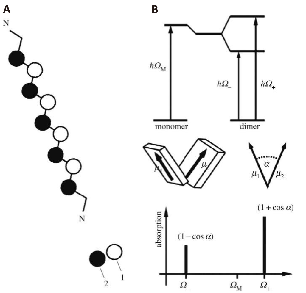
Figure 17. Scheme of a Quasilinear Polymethine Chain (A) Shown Above (Figure 9)[35,92,93,103]. Excitonic shift and splitting in molecular dimers for an alternate orientation of transition dipole moments (B)[34,62-65,103]. When the interaction of both the exciton transitions with the environment is absent, the optical absorption spectrum is given by two zero-width lines shifted relative to one another along the frequency axis (bottom right). “Switching on” this interaction results in the transformation of both zero-width lines to optical bands of a nonzero width. The optical band shape for the dimers of a polymethine dye is obtained[35] by determining the interaction of electron (exciton) transitions with the motion of nuclei of the environment[35] in the framework of the Egorov theory of molecular quantum transitions[11,37]. Reprinted (Adapted) from Ref.[103] with Permission from CC BY.

 

The shape of the optical absorption bands of polymethine dye dimers can be calculated using the formula[34,35]

 

$$ {K}_{D}=\frac{1}{2}\left[\left(1+\mathit{cos}\alpha \right){K}_{+}\left(\Omega \right)+\left(1-\mathit{cos}\alpha \right){K}_{-}\left(\Omega \right)\right]\left(89\right)$$

 

where the rate constants for the transitions to the upper and lower exciton states K+(Ω) and K_(Ω) are governed by Equations (65-85), and the directions of the transition dipole moments of monomers form angle α. Figure 18 shows an example of a theoretical explanation of the shape of optical absorption bands in dimers (D) based on taking into account exciton effects in QCM[34,35].

 

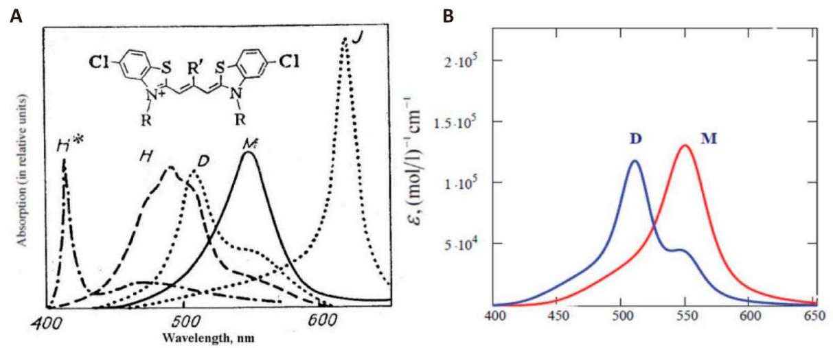
Figure 18. Theoretical Optical Absorption Band Shapes of a Thiapolymethinecyanine (B) Fitted to the Basic Experimental Data on Dye Monomers (M) and Dimer (D)[34,35] (ε is the extinction coefficient, wavelength λ=2πc⁄Ωnref) Shown in the General Picture (A) Challenging by James[21] and Herz[22]. The polymethine chain length L=6d, where d are certain roughly equal bond lengths in the chain. Absorption bands are computed by Equations (65-86) with η=1 instead of the Gamow exponent exp(-4θ⁄(1-ξ2)) when fitting them to the experimental data in terms of wavelength λmax, extinction εmax, and half-width w1⁄2 with a high degree of accuracy. The following parameters of the “monomer + environment” system are used[35]: q=1.48e, where e is the electron charge; m=3.5me, ω=5×1013s-1, d=0.14nm, nref=1.33, J1=5.4eV, J1-J2=1.42eV, E=0.21eV, γ=0.17eV, and T=298K. The following parameters of the “dimer + environment” system are used (Figure 17, Equation (89))[35]: α=61°, q=1.4e, m=3.5me, ω=5×1013s-1, d=0.14nm, nref=1.33, J1=5.4eV, J1-J2-=1.43eV, J1-J2+=1.56eV, hence the excitonic splitting energy J2--J2+≡ΔJ(D)=0.13eV, E=0.21eV, γ=0.15eV, and T=298K. Reprinted (Adapted) with Permission from The Royal Society of Chemistry.

 

James[21] and Herz[22] show classical experimental data on monomer-dimer (M‒D) concentration equilibria (see Figure 19), which are similar to classical experimental data on monomer–J-aggregate (M‒J) concentration equilibria (Section 12). These M–D concentration equilibria, like the M–J concentration equilibria, are explained on the basis of QCM (Figure 19)[35].

 

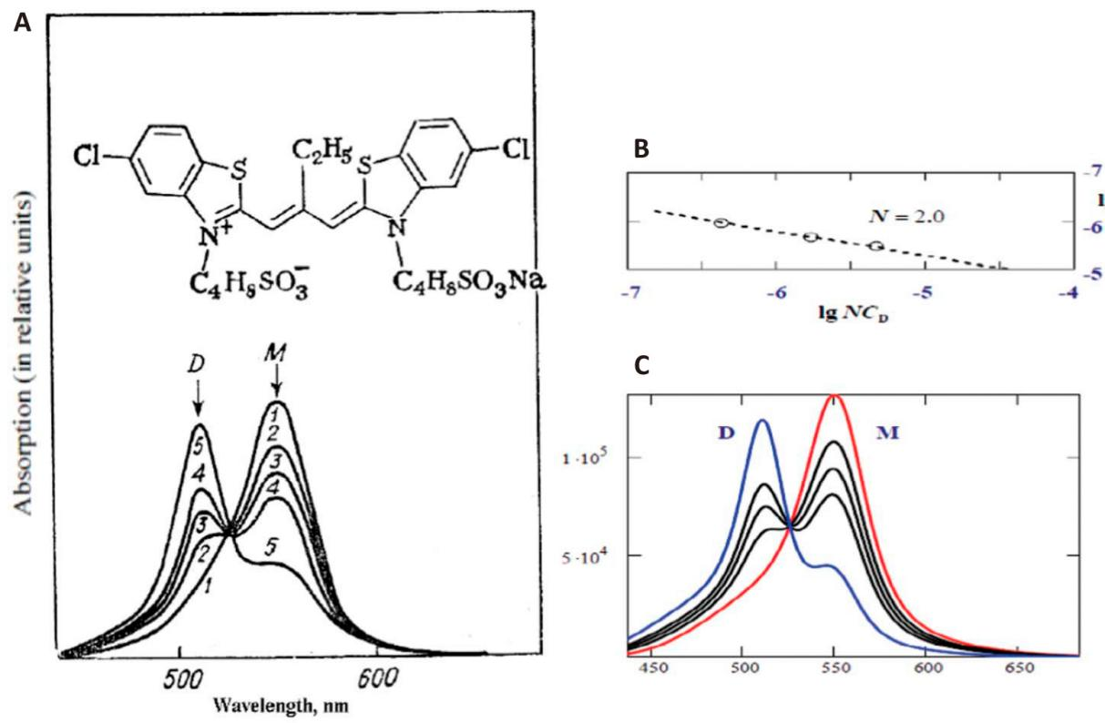
Figure 19. Optical Absorption Band Shapes for the Monomer–Dimer Concentration Equilibria of a Thiapolymethinecyanine at 25°C. Experiment (A): dye concentrations in μmol l–1 are: 1.6 in 40% MeOH (1); and 1.6 (2), 4 (3), 8 (4) and 80 (5) in water[21,22]. Theory (B and C): absorption bands of monomer (M) and dimer (D) are taken from Figure 18[34,35]. The intermediate relative concentrations of the dye converted into the D-state are: 27% (2), 43% (3) and 58% (4)[35]. Molar concentrations of the dye in the monomeric (CM) and dimeric (CD) forms are derived from absolute concentrations reported by Herz[22] (see above) and relative concentrations obtained by our fitting. They give the number of molecules N=2 in a dimer from the law of mass action (B). Reprinted (Adapted) with Permission from The Royal Society of Chemistry.

 

14.2 Broad Optical H-bands: Dozy-chaos-exciton Coupling in H-aggregates Resulting from Inelastic Binary Collisions of Polymethine Species in Solutions

The shape of the broad H-band of H-aggregates (see Figure 18) differs significantly from the shape of the D-band of dimers (not to be confused with the D-band that is a part of the J-band, see Section 8). As shown in Egorov’s study[34], the H-band can be represented as the sum of two D-bands, shifted relative to each other and included in the sum with different weights (see Equation (89) and Figure 20). Consequently, the probable optical chromophore of H-aggregates is a tetramer, the formation of which in an aqueous solution occurs in two stages.

 

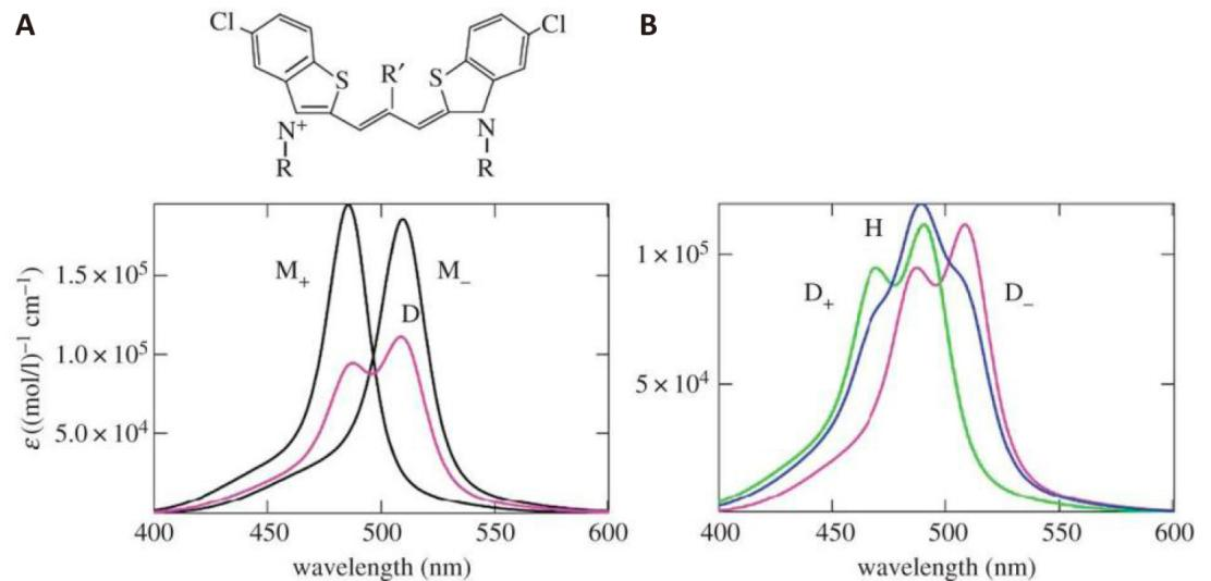
Figure 20. Theoretical Optical Absorption Band Shapes in Thiapolymethinecyanines[34] Fitted to the Available Experimental Data on H-aggregates Shown in the General Picture Presented in 1977 (Figure 18A)[21]. The polymethine chain length is L=6d, where d denotes certain roughly equal bond lengths in the chain. The absorption H-band (B) is computed from Equations (65-86) and (89) when fitting them to the experimental data in terms of the wavelength λmax, extinction coefficient εmax, and half-width w1⁄2 with a high degree of accuracy. We used the “H-aggregate + environment” system parameters[34] q≡q(H)=1.51e, m=3.5me, ω=5×1013s-1, d=0.14nm, nref=1.33, J1=5.4eV, J1-J2-=1.59eV, J1-J2+=1.68eV, hence the excitonic splitting energy J2-—J2+≡ΔJ(H)=0.09eV, E=0.19eV, γ=0.13eV, and T=298K. In (A), for the virtual D-band intermediate dimer angle αM-M=104° (see the scheme in Figure 17), εD(λ)=[(1+cosαM-M)εM+(λ)+(1-cosαM-M) εM-(λ)]⁄2. In (B), the H-band is produced by a tetramer (αD-D=94°) composed of two intermediate dimers (αM-M=104°) regarded as two novel monomers (supermonomers); εD-(λ)=εD(λ) and εD+(λ)=εD(λ+18nm); εH(λ)=[(1+cosαD-D)εD+ (λ)+(1-cosαD-D)εD-(λ)]⁄2. The large fitting angles αM-M=104°and αD-D=94° show that H-aggregates are not compact systems. Reprinted (Adapted) from Ref.[34] with Permission from CC BY.

 

At the first stage, inelastic pairwise collisions of monomers lead to the formation of dimers. In the second stage, inelastic pairwise collisions of these transient dimers lead to the formation of final tetramers. From here follows the algorithm for calculating the shape of the H-band. At the first stage, we approximate the theoretical result on the shape of the absorption band of dimers (Equations (65-86) and (89)) by varying the parameters of the system to the probable shape of the band of transient dimers (see Figure 20A). At the second stage, these transient dimers are considered as supermonomers, which are included in the theoretical result based on the shape of the absorption band of the dimers (Equations (65-86) and (89)). As a result, we obtain the desired theoretical expression for the shape of the optical absorption band of tetramers (Figure 20B). Fitting this theoretical expression to the experimental H-band is done by trial and error. The angles between the transition dipole moments of the components obtained during the fitting process turn out to be large (see caption to Figure 20), which indicates both the looseness of the structure of the H-chromophore (tetramer) and the looseness of the structure of the entire H-aggregate formed from H- chromophores connected in some way to each other. This picture differs significantly both from the picture of the ordered compact structure of J-aggregates (Figure 12) and from the picture of the structure of H-aggregates in the form of an ordered compact deck of cards reported in the literature[16,17,21,34].

 

From Figures 18 and 21, it can be seen that the agreement of the theoretical shape of the M-band, D-band and H-band[34] with the experimental data[21,22] is successful.

 

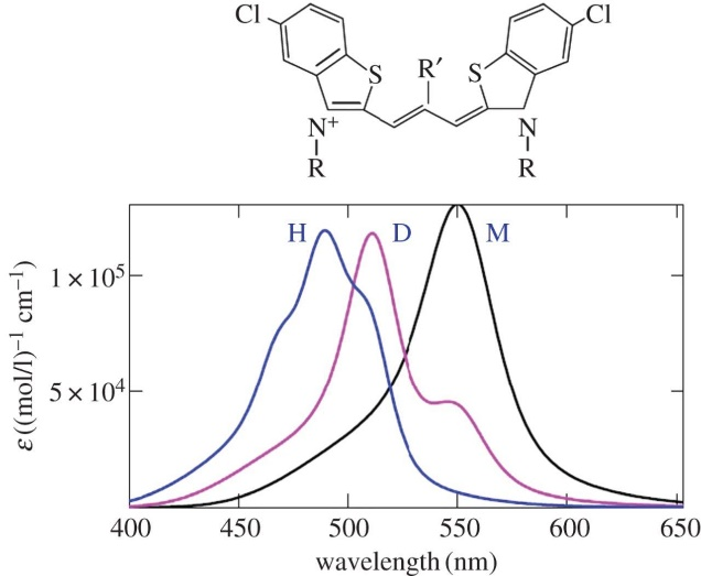
Figure 21. Theoretical Optical Absorption Band Shapes in Thiapolymethinecyanines[34] Fitted to the Basic Experimental Data on Polymethine Dye Monomers (M), Dimers (D) and H-aggregates Shown in the General Picture Presented by James[21] (Figure 18A). The parameters of the “species + environment” systems (monomer and dimer) are given above in the caption to Figure 18. The parameters of the “H-aggregate + environment” system are given above in the caption to Figure 20. Reprinted (Adapted) from Ref.[34] with Permission from CC BY.

 

14.3 Narrow Optical Band in H*-aggregates: Strong Dozy-chaos-exciton Coupling Effect

The explanation of the well-known H*-band of optical absorption[21,22], which is narrow and blue-shifted relative to the M-band, was first undertaken by Egorov[34,102,103]. This explanation is based on taking into account the structural features of polymethine dyes that form H*-aggregates. Namely, H*-monomers are cyclic bis-thiacarbocyanines, in which the polymethine chains of two identical uniplanar monomers are cross-linked at their ends by hydrocarbon radicals (Figure 22A)[22]. During the formation of H*-aggregates, this structure leads to a significant strengthening of the excitonic coupling within them. Based on the similarity of the shapes of the H*-band and the D-band obtained in the experiment (see Figure 18, for both bands the peak is in the blue part of the band, and the wing is in the red), Egorov suggested that the optical H*-chromophores in H*-aggregates are dimers (H*-dimers)[103]. The aforementioned anomalously strong exciton coupling leads to strong competition between two excitonic transitions (Frenkel exciton)[62-65], which interact with each other through the chaotic motion of reorganization of the nuclear environment. As a result, the more intense transition to the upper exciton state (see Figure 17) becomes even more organized, leading to a narrow peak in the shape of a band, and the less intense transition to the lower exciton state (Figure 17), on the contrary, becomes even more disorganized, which leads to a wide spectral wing (Figure 22B). This effect of dynamic interference of two excitonic transitions (dozy-chaos–exciton coupling effect) in H*-dimers is formally taken into account by considering the dependence of the dozy-chaos energy γ on exciton states[103]. Such a strong dozy-chaos–exciton coupling effect can be considered as a “process” in which low-organized transitions to the lower exciton state pump out dozy chaos from highly organized transitions to the upper exciton state using the Frenkel exciton. In short, highly organized excitonic transitions in optical H*-chromophores (i.e., H*-dimers) are a powerful source of dozy chaos for low-organized transitions[103].

 

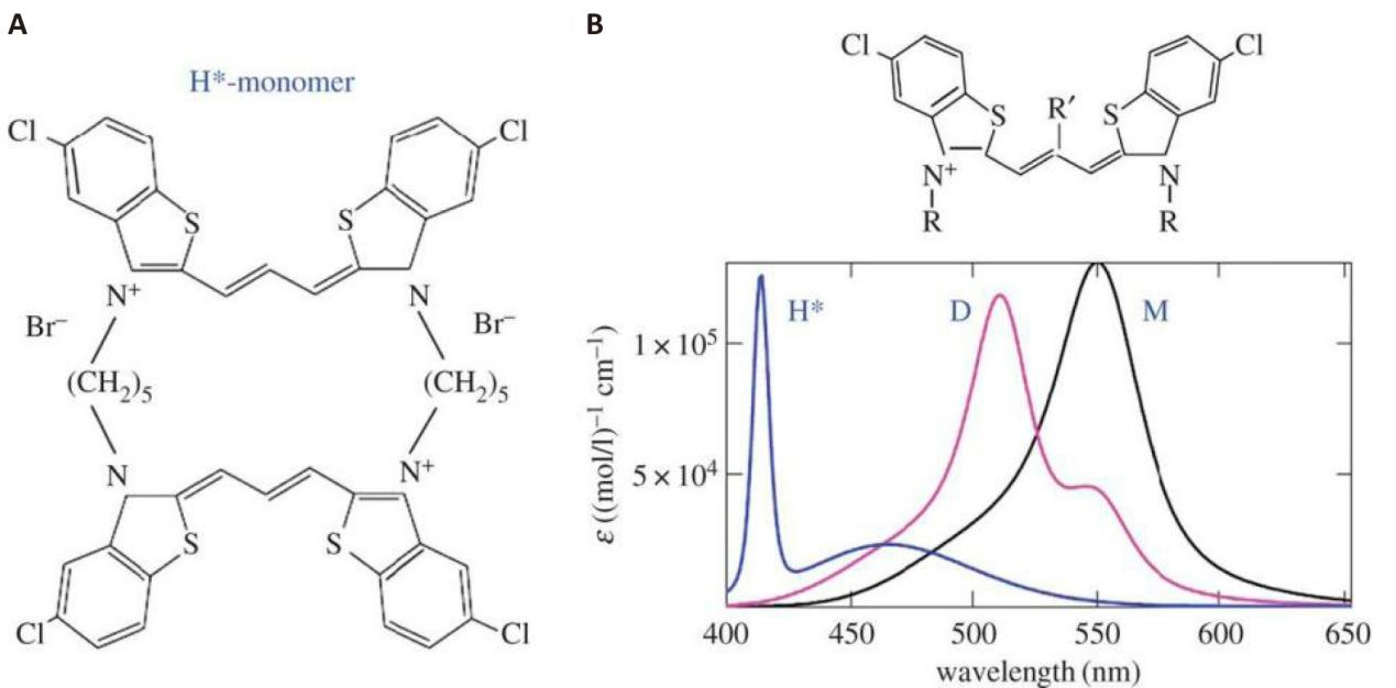
Figure 22. Theoretical Optical Absorption Band Shapes in Thiapolymethinecyanines[34,103] Fitted to the Available Experimental Data on Polymethine Dye Monomers (M), Dimers (D), and H*-aggregates Shown in the General Picture Presented in 1977 (Figure 18A)[21]. The polymethine chain length is L=6d, where d denotes certain roughly equal bond lengths in the chain. The absorption bands are computed from Equations (65-86) and (89) when fitting them to the experimental data in terms of the wavelength λmax, extinction coefficient εmax, and half-width w1⁄2 with a high degree of accuracy. The parameters of the “monomer + environment” and “dimer + environment” systems are given above in the caption to Figure 18. We used the “H*-aggregate + environment” system parameters[103] α≡α(H*)=70°, q≡q(H*)=2.26e, m=3.5me, ω=5×1013s-1, d=0.14nm, nref=1.33, J1=5.4eV, J1-J2-=1.67eV, J1-J2+=2.1 1eV, hence the excitonic splitting energy J1-J2+=ΔJ(H*)=0.44eV, E-=0.2eV, E+=0.1eV, γ-=1.16eV, γ+=0.09eV, and T=298K. Reprinted (Adapted) from Ref.[103] with Permission from CC BY.

 

In conclusion, we note that H*-aggregates are the most unstudied systems compared to other aggregates of polymethine dyes. For example, it is unknown how H*-chromophores (H*-dimers) are packaged into H*-aggregates. It cannot be ruled out that H*-aggregates are represented only by H*-dimers.

 

15 SHAPE OF OPTICAL BANDS: CONCLUDING REMARKS AND RESULTS

Let us note here that the idea of calculating the shape of the bands of H-aggregates (H-tetramers), reflecting the physical mechanism of their formation in liquid solutions (Section 14.2), can be used to interpret the more complex shape of the optical bands of some other aggregates of polymethine dyes, since they are formed as a result of inelastic multiple binary collisions of polymethine particles of varying complexity[34].

 

Finally, we show all the variety of results on the interpretation of the shape of the optical bands for different polymethine species (Sections 11, 12 and 14) in Figure 23.

 

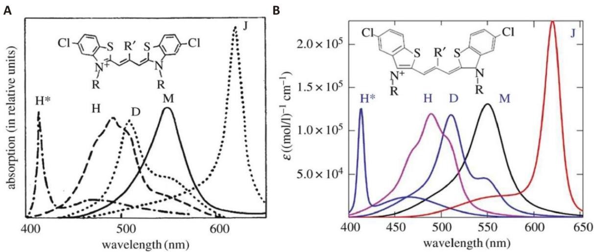
Figure 23. Optical Absorption Band Shapes in Thiapolymethinecyanines. a: Experimental data on monomers (M), dimers (D), H-, H*- and J-aggregates[21]. b: Appropriate theoretical fit to these data[34,102]. The fitting parameters for the theoretical band shapes for the monomer, dimer, H-aggregate and H*-aggregate are given above in the captions to Figures 18, 20 and 22[34]. The narrow, intense and red-shifted absorption J-band is computed from Equations (65-86) with η=1, where the “J-aggregate + environment” system parameters are[34] q≡q(J)=0.97e, m=me, ω=5×1013s-1, d=0.14nm, nref=1.33, J1=5.4eV, J1-J2=1.243eV, E=0.22eV, γ=0.088eV, and T=300K. Reprinted (Adapted) from Ref.[34] with Permission from CC BY.

 

16 EXPLANATION OF THE HARRISON ET AL. EXPERIMENT BY PETRENKO AND STEIN

Harrison et al. experimentally showed that the narrow and intense J-band of THIAMS dye[24,25] (see Petrenko & Stein[20], Table 3 therein) broadens greatly and loses intensity with a significant increase in the concentration of the dye in the solution[24]. According to Petrenko & Stein[20], this effect (Figure 24) is associated with the incorporation of additional dye monomers into the J-aggregate chromophore (Figure 12), which leads to a twofold increase in the reorganization energy E (see caption to Figure 24). Unfortunately, in Petrenko & Stein’s study[20] the structure of this modified J-chromophore is not shown.

 

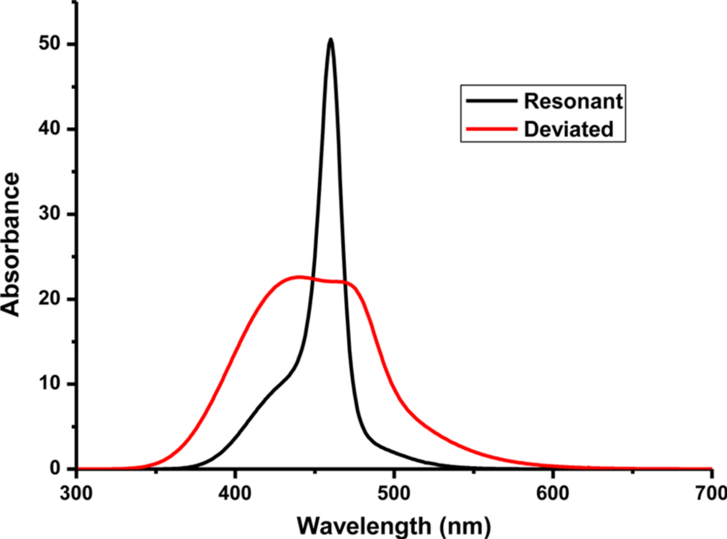
Figure 24. Change in Theoretical Spectra of J-aggregate with Deflection from the Nano-resonance Condition (Equations (29-31))[20]. Optical bands were obtained by Petrenko & Stein[20] by fitting theoretical Equations (65-85) to experimental data of Harrison et al[24]. The black line describes a J-band, consisting of L-peak and D-wing (on D-wing and L-peak see above, Section 8), with the following parameters: E=0.2eV, γ=0.11eV, L=1.68nm, J1=5.5eV, and J2=3.72eV; the red line describes a “J-band” with the following parameters: E=0.4eV, γ=0.15eV, L=2.8nm, J1=5.5eV and J2=4.0eV, here the D-wing turns out to be slightly more intense compared to the L-peak[20]. Presented theoretical spectra generate change in the sharp J-band of THIAMS dye (Table 3 in [20]) in aqueous solution at 0.80% w/w dye into a wide “J-band” at 3.53% w/w dye[24]. Reprinted (Adapted) from Ref.[20] with Permission from American Chemical Society.

 

17 J-BAND: LUMINESCENCE ASYMMETRY RELATIVE TO ABSORPTION AND ANOMALLY SMALL STOKES SHIFT

According to standard quantum theory, which does not take into account the dynamics of the transient state, the transition from absorption spectra to luminescence spectra is carried out by changing the sign of the heat energy

 

$$ \Delta \to -\Delta \left(90\right)$$

 

i.e., in Equations (70) and (71), as well as in the law of conservation of energy, Equation (85)[3,33]. Applying Equation (90) to the optical absorption bands shown, for example, in Figure 6B (Section 4), we obtain mirror-symmetrical luminescence bands shown in Figure 25.

 

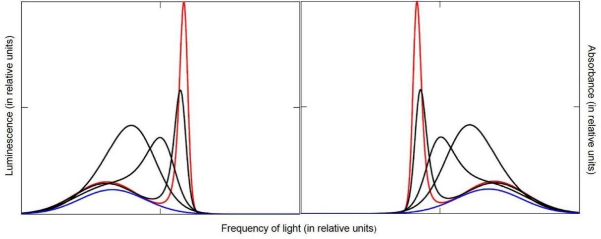
Figure 25. Standard Luminescence Symmetry Relative to Absorption. Symmetric picture of absorption[34,35] (Figure 6B) and luminescence spectra obtained by changing the sign in the heat energy Δ→-Δ (Equation (90)) in theoretical absorption spectra[33] (Equations (65-85)) according to standard quantum mechanics of condensed matter[3]. Reprinted (Adapted) from Ref.[33] with Permission from CC BY.

 

In contrast to the theoretical mirror-symmetrical picture of the spectra presented in Figure 25, the Aviv–Tischler experiment for J-aggregates in Langmuir films shows asymmetry in the absorption and luminescence spectra (Figure 26A)[26]. Structure of the corresponding dye monomer is shown in Figure 27, and the corresponding mirror-symmetric theoretical spectra are presented in Figure 26B.

 

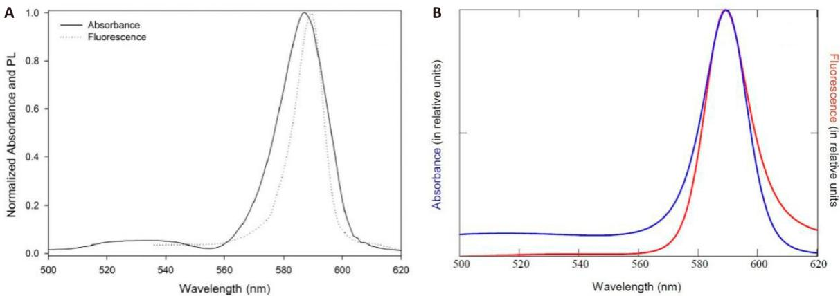
Figure 26. Comparison of Theory with Experiment for J-aggregates in Langmuir Films[33]. A: Absorption and fluorescence J-bands of a C18S4 monolayer obtained in a Langmuir film[26]; the wavelength λ=2πc⁄Ωnref. The characteristics of photoluminescence (PL) spectrum: a peak at 590nm, a FWHM=18nm, and a Stokes shift of 1nm[26]. B: Theoretical absorption and fluorescence J-bands[33], fitted to the experimental data[26] (see (A)). The absorption J-band is computed from Equations (65-85), where the “J-aggregate + environment” system parameters are m=me (me is the electron mass); nref=1.33; ω=5×1013s-1; J1=4eV; J1-J2=1.19eV; L=(6+2)d [2d lengthening the optical chromophore shown in Figure 27 due to the J-aggregation (see Figure 12)[16,17,20,33,34,36-38], d=0.14nm[16,17,20,34-38,91], LJ­(Enr)=(6+2)0.14nm=1.12nm], then we obtain E=0.349eV from the Egorov nano-resonance [Equation (29) or Equation (88), in Equation (70) parameter θ=1/2]; γ=0.092eV; η=1; and T=298K. The fluorescence J-band is symmetric to the absorption J-band and obtained from the latter by changing the sign in the heat energy Δ and increasing the energy gap J1-J2=1.19eV by 0.785eV in order for the Stokes shift to be zero (cf. Figure 25). Reprinted (Adapted) from Ref.[33] with Permission from CC BY.

 

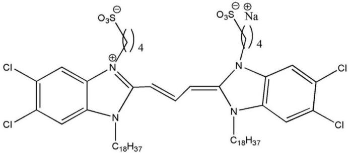
Figure 27. Structure of the Dye C18S4[33] Investigated Experimentally in Aviv–Tischler’s Study[26]. The length of the main optical chromophore, the polymethine chain[92], is defined as the distance L between nitrogen atoms N and with L=6d, where d designates roughly equal the C−C bond lengths of methine groups (cf. Figure 9), d=0.14nm[16,17,20,34-38,91]. Reprinted (Adapted) from Ref.[26] with Permission from Elsevier B.V.

 

The asymmetry of the absorption and luminescence spectra (Figure 26A) in the Aviv–Tischler experiment[26] is well reproduced (Figure 28)[33] if we follow the rules not of standard quantum theory[3] but the rules of QCM, according to which to obtain luminescence spectra from the absorption spectra, not only the sign of the heat energy Δ(Equation (90)), but also the sign of the distance L in Equations (70), (71) and (83) should be changed[33]:

 

$$ L\to -L\left(91\right)$$

 

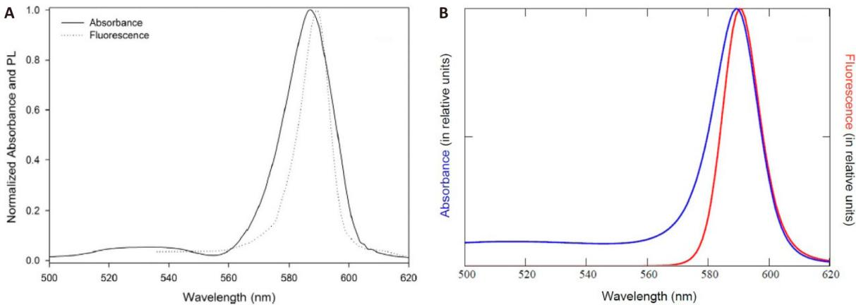
Figure 28. Comparison of Theory with Experiment for J-aggregates in Langmuir Films[33]. A: Experimental absorption and fluorescence J-bands[26] shown in Figure 26A. B: Theoretical absorption and fluorescence J-bands[33], fitted to the experimental data (see (A))[26]. The fluorescence J-band is asymmetric to the absorption J-band and obtained from the latter by changing the sign both in the heat energy Δ and in the J-chromophore length L, and  increasing the energy gap J1-J2=1.19eV by 0.785eV in order for the Stokes shift to be 1nm (cf. Figure 26B) due to the spontaneous dynamic loosening of the excited electronic state immediately before the light emission by the electron (see below). The rest of the fitting parameters are the same as those in Figure 26B. Reprinted (Adapted) from Ref.[33] with Permission from CC BY.

 

The more significant narrowness of the luminescence J-band compared to the absorption J-band and its asymmetry with respect to it can be explained by a higher degree of organization of the dynamics of the electron‒phonon transient state during luminescence compared to the dynamics during absorption[33]. Namely, the π-electronic system, as it were, learns, remembering, through interaction with the environment, its route of movement when the system is optically excited, therefore, in the process of removing this excitation, knowing this route, it behaves in a more organized manner.

 

Confirmation of the higher degree of organization of the dynamics of the electron‒phonon transient state in the luminescence process compared to the dynamics in the absorption process is the suppression effect of the M-luminescence band compared to the J-luminescence band in a mixture of monomers and J-aggregates in an aqueous solution (see Figure 29)[26,33]. This effect is explained by a much greater enhancement of the dynamic self-organization of QCT in J-aggregates than in monomers, as a result of the transition from optical absorption to luminescence[33]. In short, the “dynamic memory” of J-aggregates is much better than that of the individual dye monomers they contain.

 

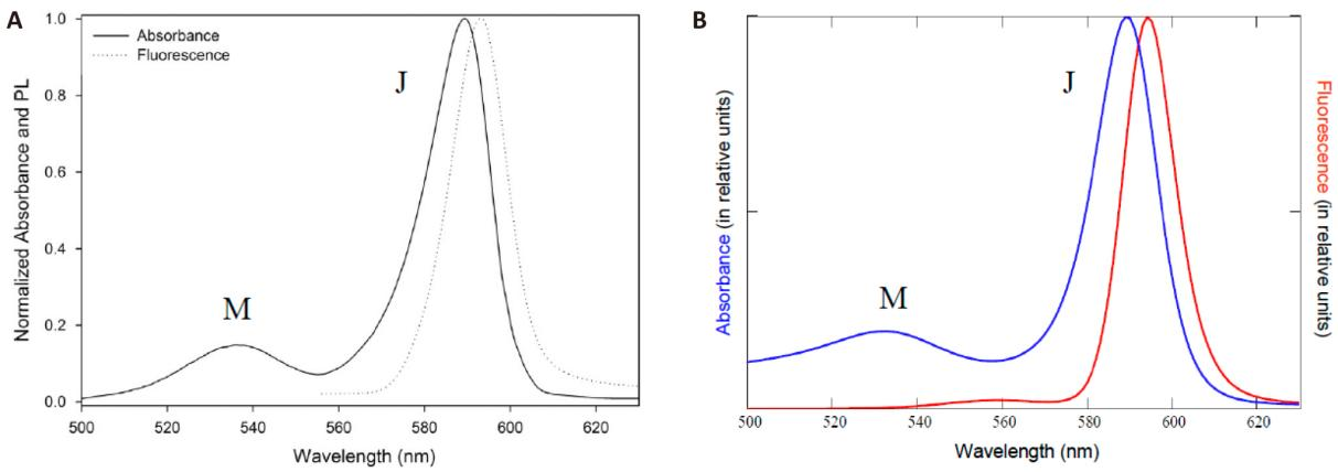
Figure 29. Experimental[26] (A) and Theoretical[33] (B) Absorption and Fluorescence Spectra of a C18S4 Aqueous Solution[26]; the wavelength λ=2πc⁄Ωnref. Luminescence: Effect of Suppression of the M-band by the J-band in an Aqueous Solution “Monomers + J-aggregates”. The absorption spectrum shows a pronounced J-aggregate peak and weak monomer shoulder. The J-aggregate absorption peak is at λ=589nm with a FWHM=18nm. The PL spectrum shows only J-aggregate emission[26], peaked at λ=594nm with FWHM=15.5nm. The absorption M-band is computed from Equations (65-85). We used the “monomer + environment” system parameters[33] m=1.6me, where me is the electron mass; nref=1.33; ω=5×1013s-1; J1=4.3eV; J1-J2=1.34eV; L=6d (L is the length of the main optical chromophore in the monomer dyes—the polymethine chain), where d denotes certain, roughly equal bond lengths in the polymethine chain of the monomers of the dye (the C−C bond length of a single methine group, d=0.14nm[16,17,34-38,103], see the caption to Figure 27 above); E=0.33eV [in Equation (70) parameter θ=0.433]; γ=0.168eV [in Equation (70) parameter θ0=1.97]; T=298K; and η=0.7.[33] The fluorescence M-band is obtained from Equations (65-85) for the absorption M-band by changing the sign in the heat energy Δ and in the distance L, and increasing the energy gap J1-J2=1.34eV by 0.76eV due to the spontaneous dynamic loosening of the excited electronic state immediately before the light emission by the electron (see below). The fitting parameters for both J-bands (B) are given in Figure 26B above (where it is assumed that the tunnel factor η=1), the exceptions are η=0.7 and the energy gap J1-J2=1.19eV increased by 0.781eV (the Stokes shift is 5nm) due to the aforementioned spontaneous dynamic loosening of the excited electronic state[33]. The admixture of monomers with respect to J-aggregates in an aqueous solution of the dye is assumed to be 20%. With this relative monomer concentration, the theoretical M-band is noticeable only on the shortwave wing of the absorption band and practically not noticeable on the shortwave wing of the luminescence band. Reprinted (Adapted) from Ref.[33] with Permission from CC BY.

 

The very small value of the Stokes shift (Figures 28 and 29) is explained by two effects[33]. The first effect is associated with the convergence of Egorov nano-resonances associated with absorption and luminescence, as a result of an anomalously high degree of regularization of mixed, chaotic and regular, transient states (Figure 25). Formally, a high degree of regularization corresponds to a very low dozy-chaos energy γ. The second effect is associated with an anomalously strong loosening of the excited π-electronic state due to its large extent. This leads to an anomalously high energy of the excited state and, as a consequence, to the emission of a J-aggregate with an anomalously high frequency of light[33].

 

18 SHAPE OF ONE- AND TWO-PHOTON RESONANCE BANDS IN POLYMETHINE DYES

Figure 30 shows the experimental shapes of optical bands of one-photon and two-photon absorption of a certain polymethine dye (Figure 31) in a solvent—chloroform[133]. In the case of one-photon absorption, the band is quite narrow and intense, so we can assume that it corresponds to the Egorov nano-resonance. Upon transition to two-photon absorption, the band shape sharply deteriorates[133], which is associated with a strong violation of nano-resonance conditions.

 

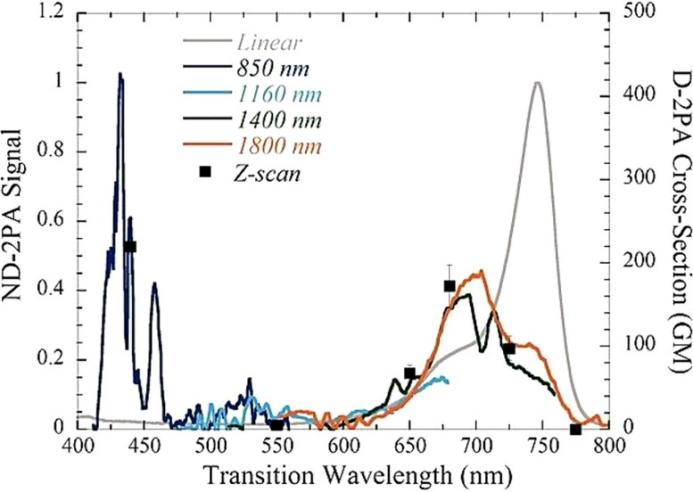
Figure 30. Nondegenerate 2PA Spectra for a Solution of Selenopyrylium-terminated Polymethine Dye Se-3C Dissolved in Chloroform. Different pump wavelengths were used to observe the full ND-2PA spectra. Solid circles are degenerate 2PA (D-2PA) cross sections derived from femtosecond-pulsed Z-scan measurements. 1 GM is defined as 1×10–50cm4 s photon–1. Experimental uncertainties in the values were estimated to be ±10%. The linear absorption spectra are shown as reference. Reprinted (Adapted) from Ref.[133] with Permission from American Association for the Advancement of Science.

 

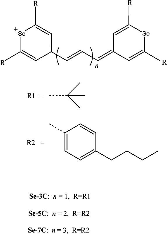
Figure 31. Chemical Structure of Selenopyrylium-terminated Polymethine Dye Cations [18,133]. The monovalent counterion is not shown. Reprinted (Adapted) from Ref.[133] with Permission from American Association for the Advancement of Science.

 

In Figure 32, both of these experimental band shapes are modeled within the framework of quantum–classical mechanics (see Section 6, Equations (65-85))[18,19].

 

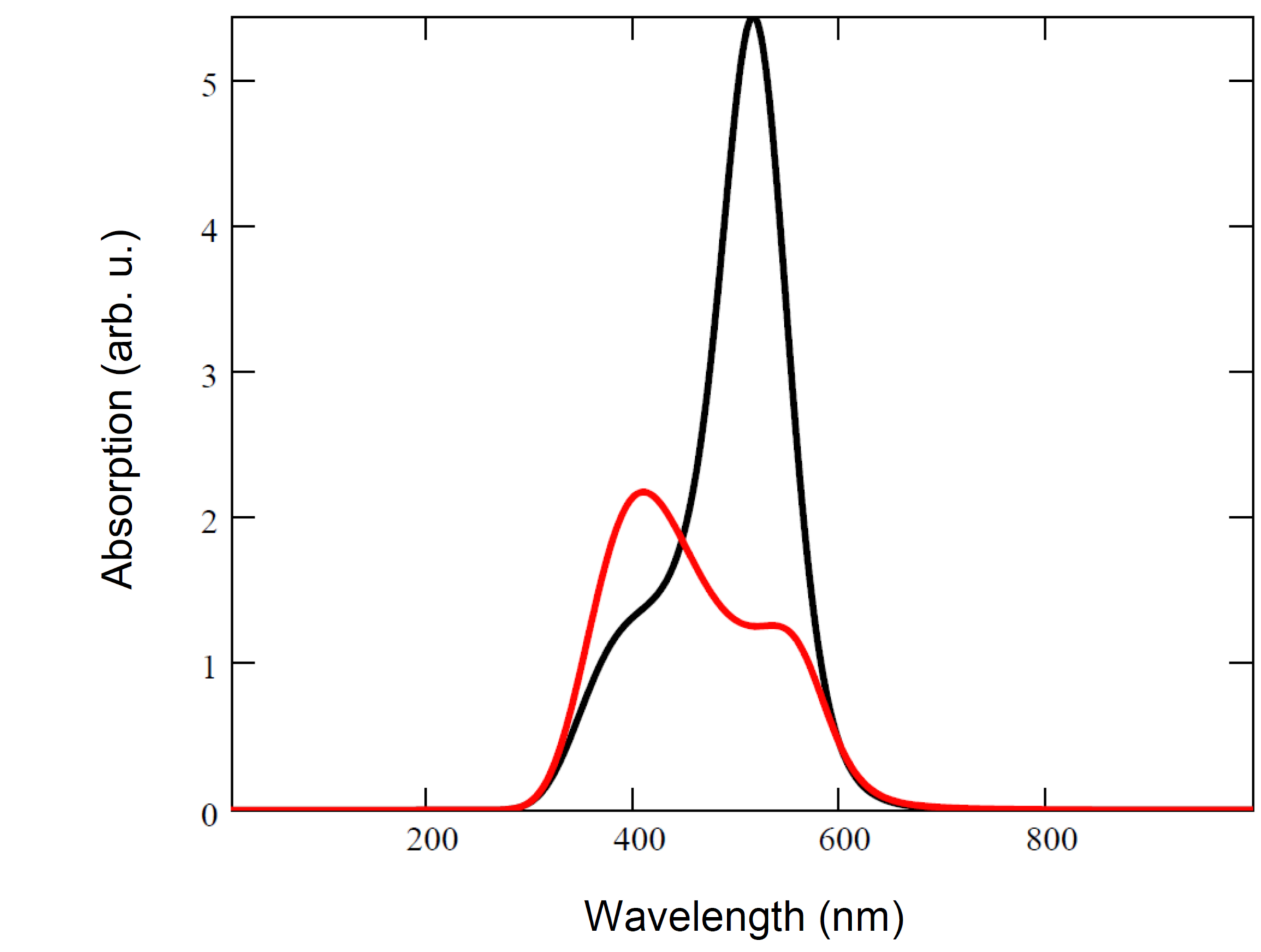
Figure 32. Transformation of the Theoretical Spectra of a Model Polymethine Dye with Different Deviations from the Nano-Resonance Condition θ=1/2 (see Equatios (29-31) and (88), in Equation (70) parameter θ=1/2)[18,19]. The optical band that is near the nano-resonance band (black curve) corresponds to θ=0.44, the optical band that is far beyond the nano-resonance band (red curve) corresponds to θ=0.88. Both bands are computed from Equations (65-85), where the “dye + environment” system parameters are m=me (me is the electron mass); nref=1.33; ω=5×1013s-1; J1=5eV; J1-J2=0.5eV; E=1eV; Lblack=0.384nm; Lred=2Lblack; γblack=0.45eV; γred =0.34eV; and T=298K. Reprinted (Adapted) from Ref.[18] with Permission from CC BY.

 

The strong violation of the Egorov nano-resonance conditions during the transition to two-photon absorption is easy to understand if the shape of the bands shown in Figure 32 in wavelength coordinates along the abscissa axis, depict in photon energy coordinates (see Figure 33)[19].

 

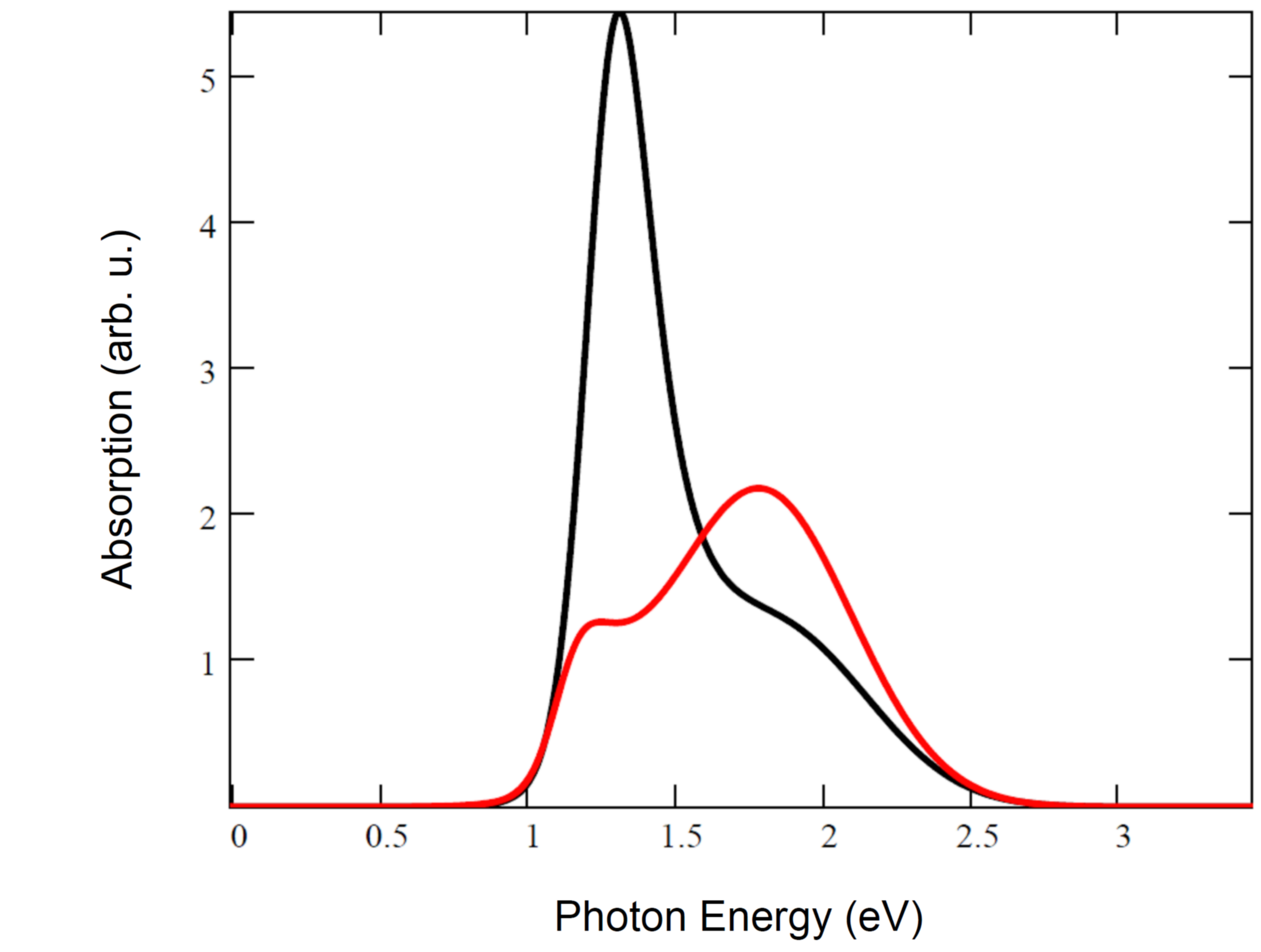
Figure 33. The Theoretical Spectra in Figure 32 are Shown in Photon-energy Coordinates for Convenience of Discussion[19]. Additionally, for convenience, it is assumed that the energy gap J1-J2≡0. Reprinted (Adapted) from Ref.[19] with Permission from Elsevier B.V.

 

Under resonant conditions with one-photon absorption, we can say that single acts of absorption of photon energy occur most likely in the region of the peak of the band and with less probability in the region of its wing (Figure 33). When going from resonant one-photon absorption to two-photon absorption, a significant shift occurs in the main region of photon absorption, namely from the low-energy peak of the band to its high-energy wing (Figure 33)[19].

 

This shift can also be explained based on the law of conservation of energy (Section 6, Equation (85)):

 

$$ \hslash \Omega ={J}_{1}-{J}_{2}+\Delta $$

 

which for two-photon absorption is rewritten as[19]

 

$$ 2\hslash \Omega ={J}_{1}-{J}_{2}+\Delta \left(92\right)$$

 

Let’s rewrite the law of conservation of energy for the case of the act of absorption of a single photon (Equation (85)), substituting the energy of reorganization of the nuclear subsystem E instead of heat release Δ[19]:

 

$$ \hslash \Omega ={J}_{1}-{J}_{2}+E\left(93\right)$$

 

The physical meaning of this equality is obvious: the energy of the photon ℏΩ is spent on the electronic excitation energy J1-J2 and on the reorganization energy of nuclei E. Then for two-photon absorption from Equation (92) we have similarly[19]

 

$$ 2\hslash \Omega ={J}_{1}-{J}_{2}+{E}^{\text{'}}\left(94\right)$$

 

where

 

$$ {E}^{\text{'}}=E+\delta E>E\left(95\right)$$

 

To estimate the two-photon nuclear reorganization energy E', we can set

 

$$ \delta E\cong E\left(96\right)$$

 

that is

 

$$ {E}^{\text{'}}=2E\left(97\right)$$

 

Thus, replacing the nuclear reorganization energy E with 2E in nano-resonance, that is, replacing the parameter ,

 

$$ \theta \equiv \frac{{\tau }_{e}}{\tau }=\frac{E L}{\hslash \sqrt{2{J}_{1}/m}}\left(98\right)$$

 

(Equations (29-31) and (70)), with the parameter θ=1, during the transition from one-photon to two-photon absorption, shifts the physical system far beyond the resonance limits. This can be interpreted as a “parasitic” pumping of dozy chaos by a quantum–classical electron[11,19,33] from the wing of the J-band to its peak (see Figure 32, θ=0.44≅0.5 and θ=0.88≅1). Thus, important experimental data[133] on two-photon absorption (see Figure 30) find their explanation.

 

To return a system with parameter θ=1 to the resonance desired in applications, but under new conditions of two-photon absorption, it is necessary to reduce the product E⋅L by a factor of 2 (see Equation (98), and Figure 32 with θ≅1 and θ≅0.5)[19]. In other words, under experimental conditions it is necessary to reduce the polarity of the medium corresponding to the reorganization energy E and/or the length L of the polymethine chain, which is the main optical chromophore.

 

Figures 34 and 35 illustrate the conditions for the restoration of the Egorov nano-resonance by studying the dependence of the shape of the model two-photon absorption band on the reorganization energy E[19]. According to the result in Figure 34, to restore nano-resonance, the reorganization energy E=1eV (red) must be reduced to E=0.6eV (magic). According to the result in Figure 35 nano-resonance under the conditions of a two-photon experiment is red-shifted and should be sought using a non-polar solvent, somewhere on the border of the red and infrared regions, or in the near-infrared region[19].

 

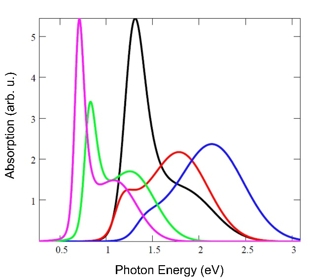
Figure 34. Transformation of the Theoretical Band Shape for the Two-Photon Absorption (Figure 33, Red Curve) with Varying the Reorganization Energy E[19]. θ0≡Ered⁄γred≡constant=2.94; E=1.2eV (blue), 1eV (red), 0.7eV (green), 0.6eV (magic). The magic band shape corresponds to the restored Egorov nano-resonance. Reprinted (Adapted) from Ref.[19] with Permission from Elsevier B.V.

 

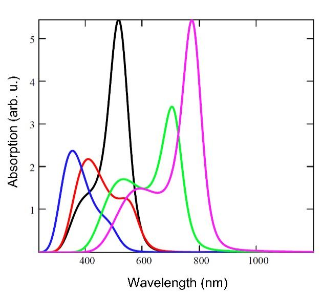
Figure 35. The Same as in Figure 34, Except for the Wavelengths on the Abscissa Axis[19]. Reprinted (Adapted) from Ref.[19] with Permission from Elsevier B.V.

 

The nano-resonance shift to the red region of the spectrum as a result of the transition from one-photon to two-photon absorption with a decrease in the reorganization energy E is qualitatively explained in a similar way to the explanation of the corresponding shift of the optical band with a decrease in length L in Figure 7 (see Section 6).

 

19 ADVANTAGES OF QCM IN EXPLAINING THE SHAPE OF OPTICAL BANDS

The excitonic approach uses a large number of fitting parameters (sometimes more than ten; see, e.g., the paper by Didraga et al.[134]), including some that are difficult or impossible to directly measure or calculate (e.g., diagonal disorder, disorder correlations, intermolecular interactions). This significantly reduces the real value of the calculation results for specific J- and H-aggregates obtained within the framework of the excitonic model.

 

The situation is quite different with the quantum-classical approach. It uses only one fitting parameter, which is not yet amenable to direct measurement or calculation—the dozy-chaos energy γ. The remaining parameters, such as the binding energy of an electron in the excited and ground states or the reorganization energy of the environment, are in principle possible to calculate using modern methods of quantum chemistry. Moreover, the binding energy can be obtained directly in experiment[135-137], and the energy of nuclear reorganization can be estimated using a simple resonance formula (see Section 13, Equation (88)):

 

$$ {E}_{\text{Enr}}=\frac{\hslash \sqrt{{J}_{1}/2m}}{{L}_{\text{Enr}}}\left(99\right)$$

 

Moreover, there is a fairly clearly defined range of dozy-chaos energies γ. The energy γ is approximately 1–3 times higher than the energy of nuclear reorganization under normal conditions of chemical kinetics (see Section 4, caption to Figure 6), and it is approximately 0.2 of the energy of nuclear reorganization under conditions of the J-band effect (see Section 4, caption to Figure 6 and Section 12, caption to Figure 11).

 

As noted in Section 3.5, exciton theory does not provide a connection between band shape and well-defined physical parameters of the system that can be calculated and/or measured. For example, the exciton theory does not include such an important and physically transparent quantity as the energy of nuclear reorganization, which arises during electronic transitions due to electron‒phonon and exciton‒phonon interactions. This fact alone is enough to reduce the exciton theory to the level of “science fiction”.

 

Based on the half-width w1⁄2 of the most intense (resonant) optical absorption band in the series of Brooker et al.[123] (see above, Section 11, Figure 10) and estimated using the standard quantum‒mechanical Marcus formula (Section 7, Equation (87))

 

$$ {w}_{1/2}=2\sqrt{2\mathit{ln}2}\sqrt{2{\lambda }_{r}{k}_{B}T}\approx 0.09{e}{V}\left(100\right)$$

 

(T=300K), the Marcus reorganization energy is λr≈0.03eV(λr≡2E), and according to the estimate of the Egorov nano-resonance (see Equation (99), where L=1.4nm and J1≅5eV), to which the indicated resonant optical band corresponds, this reorganization energy is λr≈0.63eV[34,38]. This value, 21 times (!) higher than the generally accepted value, was confirmed by quantum chemical calculations in the work of Petrenko & Stein[20]. Note that the fact of the fundamental importance of molecular reorganization energy as a key parameter of the theory is directly reflected by Petrenko & Stein in the titles of both of their articles on QCM: “Molecular Reorganization Energy as a Key Determinant of J-Band Formation in J-Aggregates of Polymethine Dyes” and “Toward a Molecular Reorganization Energy-Based Analysis of Third-Order Nonlinear Optical Properties of Polymethine Dyes and J-Aggregates”[18,20].

 

Another undeniable advantage of the quantum-classical approach is that the theoretical result on the shape of the J-band has the form (albeit complex) of an analytical formula, fully expressed in terms of elementary functions (Section 6). This can be easily calculated using a personal computer. At the same time, the excitonic approach requires cumbersome numerical calculations on supercomputers, even when using the smoothing technique (Sections 3.1.3.3 and 3.1.3.4)[75,78].

 

The quantum-classical approach, applied to the theoretical processing of the known Herz data (Section 12), made it possible for the first time to explain experiments on J-aggregation with increasing dye concentration in solution. These classic experiments[29-32] remain relevant[138].

 

For each concentration level, there is a thermodynamically reversible equilibrium between the monomeric and J-aggregated forms of the dye, which is reflected in the existence of an isosbestic point (see Figure 11). It should be emphasized that these classical experiments cannot, in principle, be considered theoretically within the framework of the existing excitonic model. Our theoretical interpretation reproduces the spectra of both J-aggregates and monomers for different dye concentrations (Figure 11). Also, the quantum-classical theory makes it possible to reproduce the isobestic point and its position with a high degree of accuracy (3-4%, cf. Figure 11A and Figure 11B). These results clearly demonstrate the undeniable advantage of the quantum-classical approach compared to the excitonic approach.

 

We also note that experiments on the joint study of the J-absorption band and the J-luminescence band are explained only within the framework of the quantum-classical approach (Section 17). Within the framework of the exciton approach, such an explanation does not exist. The quantum-classical approach also makes it possible to explain the parasitic effect of destruction of nano-resonance during the transition from one-photon to two-photon absorption in polymethine dyes, as well as to clarify the conditions for the restoration of this resonance (Section 18).

 

It should be emphasized that quantum–classical mechanics, supplemented by taking into account the effects of the Frenkel exciton, makes it possible to explain the shape of the optical bands of dimers, H-aggregates and H*-aggregates of polymethine dyes (Sections 14 and 15, Figure 23)[34]. However, excitonic effects do not play a role in the formation of the unique properties of the J-band of J-aggregates, its anomalously small width and anomalously high intensity[34].

 

Unfortunately, the statistical exciton theory of the J-band[73] based on the adiabatic approximation, the Franck-Condon principle and the static disorder paradigm (Section 3.1), as well as all the more recent studies in its context, are nothing more than big hoaxes, which are often encountered in the history of science and seem inevitable. In the past, the author of the article himself actively participated in its creation[75-78]. Author’s previous position was not rooted in the impeccable physical basis of the exciton theory of the J-band, but in the inertia of traditional concepts and the absence of an acceptable alternative.

 

The first approach to interpreting the J-band, based on Frenkel’s exciton theory, assumes the degradation of all characteristic features of the optical spectrum of monomer molecules in the J-aggregate. A new, opposite approach is based on a new theory—quantum–cassical mechanics of elementary electron transfers in condensed matter and assumes the development of a characteristic (resonant) feature in the spectra of polymethine dye monomers as a result of their J-aggregation. The assumption of such a development of the resonant band, i.e. enhancement of nano-resonance, is a consequence of the fact that, in contrast to the excitonic approach, the quantum–classical approach explains not only the shape of the J-band of J-aggregates, but also the shape of the optical bands of the constituent molecules of the J-aggregate.

 

20 FROM NANOPHYSICS TO MOLECULES OF LIFE AND LIVING MATERIALS

As shown above, one of the theoretical foundations of nanophysics is a new fundamental theory—quantum–classical mechanics, which takes into account the chaotic dynamics of the transient state during electron–phonon transitions[11,15,41]. In classical mechanics and classical physics, the statistical properties of particles are secondary to their dynamic properties, since they are associated only with ensembles of particles. In the microcosm, quantum mechanics refutes this idea. Namely, a certain fundamental physical quantity characterizing the statistical properties of an individual microparticle (wave function) obeys a dynamic equation (Schrödinger equation). This paradigm is in direct contradiction with the paradigm of classical physics. In quantum–classical mechanics, this remarkable paradigm of quantum mechanics finds its development in the form of the dozy chaos paradigm. That is, microparticles are characterized not only by “innate” statistics, but also by the “innate” chaotic nature of their interactions in molecules, molecular systems, in condensed matter and in other complexly organized physical systems where chaotic movement is intricately entangled in regular movement (Figure 36).

 

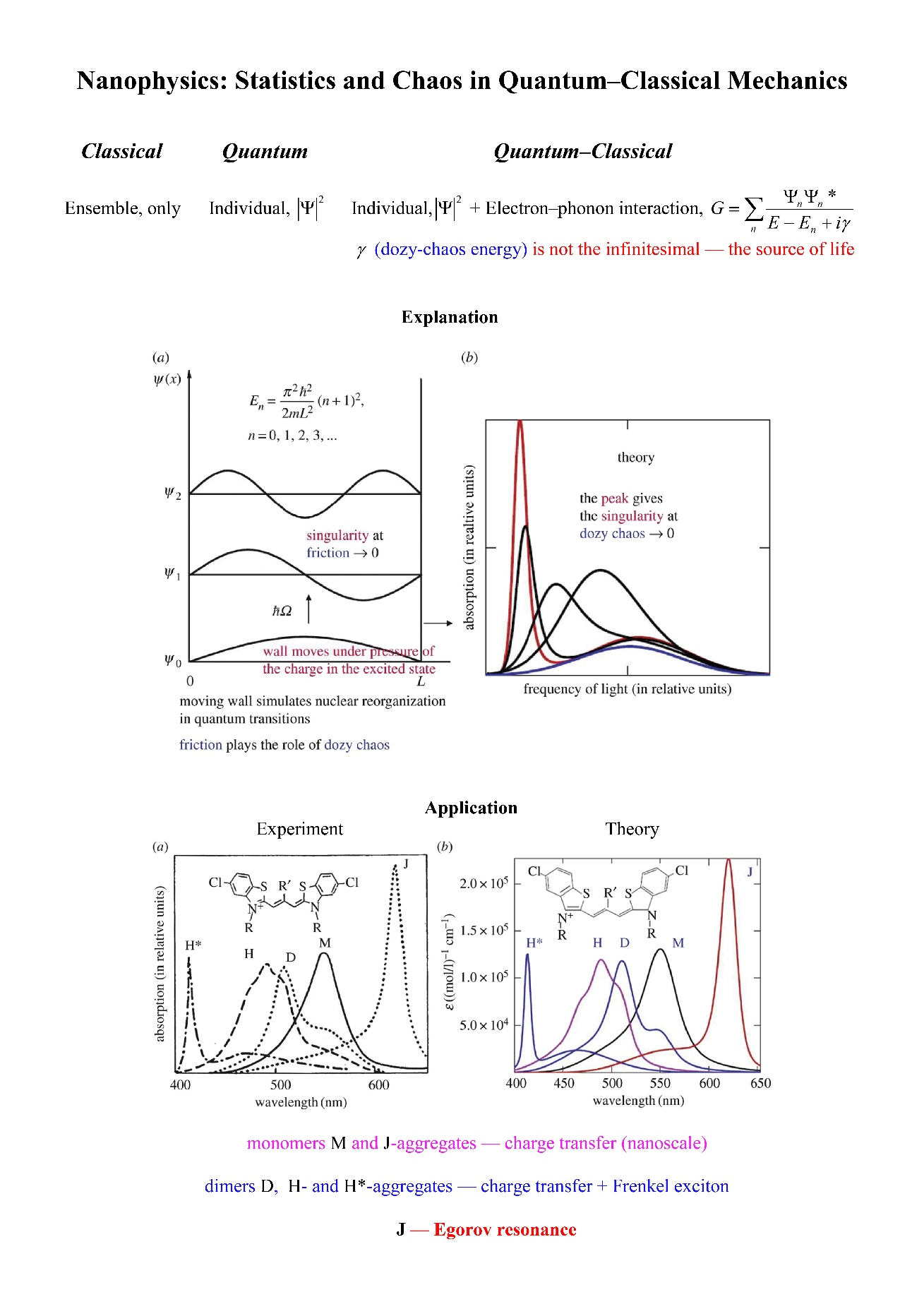
Figure 36. Quantum-classical Nano-mechanics Highlights.

 

In molecules, chaos (dozy chaos) in the interaction of electrons and nuclei always exists, but it manifests itself mainly in the process of molecular transitions (in the transient molecular state), when a reorganization of both the electronic and nuclear subsystems occurs. In the ground and excited states, which can be considered in the Born‒Oppenheimer adiabatic approximation, dozy chaos can be neglected. In the case of strong dozy (transient) chaos, quantum–classical mechanics gives the same result as the standard Franck–Condon picture of electron‒vibrational transitions (Sections 2, 7 and 9)[47]. Dozy chaos ensures the convergence of a series of time-dependent perturbation theory in quantum mechanics, which is absent in the standard quantum mechanics of molecular transitions (Section 4)[11]. In the case of weak dozy chaos, an important result of quantum–classical mechanics is the Egorov nano-resonance (Sections 3.4, 8 and 13; Figure 36), which is associated with the appearance of pronounced regular dynamics against the background of dozy chaos, and which explains the nature of the narrow and intense optical J-band of the well-known J-aggregates (Sections 11 and 12, Figure 36)[15-20,37,38,49]. The discovery of quantum–classical mechanics and Egorov’s nano-resonance opens up the possibility of creating optical spectroscopy of extended molecular systems of the order of nanometers or more, in which, along with dozy chaos, the effects of regular dynamics in the transient state appear. Dozy chaos in the transient state is provoked by a light electron “in order” to ensure the reorganization of the very heavy nuclear subsystem, and hence the very possibility of electron‒vibrational transitions. This organizing property of the electron undoubtedly plays a huge role in biological processes. The next stage in the development of quantum–classical mechanics may be the complication of the system through the organization of various aggregates (see some examples in Figure 37)[139], where the “elementary cell” in the fundamental theory and/or the starting point for the development of the theory will be the already analytically solved problem of elementary electron transfers in quantum–classical mechanics[11]. The goal of such complication and enumeration of all possible options for aggregation will be to search for the “molecule of life,” that is, quite complex, but “minimal” structural configurations in which elements of self-organization, both structural and dynamic, observed in theoretical optical spectra are clearly manifested[139]. The “atom of life” here is the quantum-classical electron itself, causing dozy chaos (Figure 36)[139]. The prototype of such an organization of the “molecule of life” is the self-organization of the living peak (L-peak, Section 8)[20,37] of the Egorov nano-resonance and/or highly dynamic self-organization of QCT in J-aggregates, leading to the formation of a narrow and intense optical J-band (Section 12, Figure 36)[15-20,37,38,49]. Thus, by increasing the complexity of the design of molecular systems, QCM opens up great prospects for the search and study of simple, alternative forms of life and related phenomena (see below, Section 21)[139]. For example, a new type of possible materials, “living materials”, could provide us with much more comfortable living conditions[139].

 

Figure 37. Examples of Schemes of Possible Aggregates in the Solid Surface and in Solution.

 

Due to the linearity of the Hamiltonian of the electron‒phonon interaction in the theory of elementary electron transfers (Section 5, Equation (43)), the above problem can be solved by analytical methods, using and developing the already created mathematical technique of generating functions (Section 5)[11]. In QCM, in particular, in the theory of elementary electron transfers, the dozy chaos in the electron‒phonon interaction is introduced not into the Hamiltonian, but into the complete Green’s function of the system, namely by replacing the infinitesimal imaginary addition in its energy denominator with a finite value (Section 5, Equations (43) and (45); Figure 36)[11,41]. This simple procedure makes it possible to introduce chaos into quantum mechanics without resorting to excessive complication of its mathematical apparatus.

 

21 ON THE PHYSICAL NATURE OF LIFE AND ITS ALTERNATIVE FORMS

The discovery of the physical source of life within the framework of QCM (Section 20, Figure 36) opens up a fundamental possibility for constructive elucidation of the nature of life and its possible alternative forms not only at the biochemical level, but also at the physical and physicochemical levels. The existing interest in the problem of the origin of life and its possible alternative forms is briefly reflected in this section.

 

Explaining the origin of our form of life is perhaps the central and most challenging issue in modern science. A new hypothesis about the origin of life on Earth has been proposed in a recently published paper[140]. The new hypothesis is based on the assumption that during the origin of life, evolution must have first employed autocatalytic systems, which only later acquired the capacity for genetic inheritance. In addition, key abiotic and early biotic molecules necessary for the formation of early life, such as cofactors, coenzymes, nucleobases, prosthetic groups, polycyclic aromatic hydrocarbons, some pigments, etc., are poorly soluble in aqueous media. To avoid the latter concentration problem, the new hypothesis suggests that life may have originated in non-polar or low-water systems, or at the interface between the non-polar and polar aqueous phases, from where it was subsequently transferred to aqueous media. To support their hypothesis, the authors of the article suggest that hydrocarbons and oil on Earth are of abiotic origin[140].

 

There is an opinion that “life is a self-replicating, evolving system expected to be based on organic chemistry”[141]. It is quite well founded, based on the knowledge that we have in the field of biochemistry, and on the practice that we have on planet Earth. In particular, it can be assumed that the structural basis of life is carbon, which easily participates in the formation of chemical bonds with many other atoms, thereby providing the chemical versatility necessary for the reactions of biological metabolism and reproduction[141].

 

Another viewpoint suggests that carbon-hydrogen-oxygen-nitrogen-based life is not the only plausible biochemistry, and in particular that the terrestrial biochemistry of nucleic acids, proteins, and sugars is probably not universal[142]. Specifically, the nature of the fluid in which life evolves determines the most suitable chemistry. Liquids other than water may be abundant on cosmic scales and may therefore be environments in which non-terrestrial biochemistry could evolve[142]. The “ammonochemistry” of the internal oceans of the Galilean moons and the “silicon biochemistry” of liquid nitrogen would have different chemical signatures than terrestrial biochemistry.

 

Estimates using plausible assumptions about the rapidity of the origin of life on early Earth suggest that it is possible that life arose from non-life on Earth more than once[143]. Multiple genesis can result in sequential independent biologies or multiple simultaneous biologies. For example, alien microbes may exist on Earth today and remain undetected by our best efforts[143]. This view is supported and developed by Cleland CE and Copley SD[144]. Strategies for searching for evidence of the shadow biosphere are outlined by Davies et al[145].

 

The article by Benner[146] discusses various definitions of life. In particular, it discusses how the very definition of life, based on Darwinian evolution, may change as supra-Darwinian species emerge, including in our descendants, as our species improves itself using technological progress. It discusses the extremely small chances of our encountering supra-Darwinian species during space exploration[146].

 

NASA’s Astrobiology Roadmap addresses three core questions[147]: How does life originate and evolve, does life exist elsewhere in the Universe, and what is the future of life on Earth and beyond? Effective and objective strategies to search for biomarkers, and evidence for a second genesis, on planets with Earth-like environments are built based on a principle of chance and necessity in biochemistry[148].

 

According to Qian et al.[149], compressed compounds of nitrogen and hydrogen (nitrogenous hydrogens), existing in a thermodynamically stable state, can produce a much more diverse chemistry than hydrocarbons, the known diversity of which provides enormous biological variability. There are a great many nitrogenous hydrogens in the Universe. Thus, the planets Uranus and Neptune consist of 8% ammonia (belonging to the simplest nitrogenous hydrogens), of which there is much more than on Earth[149].

 

In the article by Stevenson et al.[150] a new type of membrane consisting of small organic nitrogen compounds is proposed that is able to form and function in liquid methane at cryogenic temperatures. Similar stable cryogenic membranes may arise from compounds observed in the atmosphere of Saturn’s moon Titan, known for the existence of seas of liquid methane on its surface[150].

 

The first spectroscopic detection of vinyl cyanide (C2H3CN) in the atmosphere of Titan is reported, which is the best candidate for the molecule responsible for the formation of cell membranes/vesicular structures in the hydrocarbon-rich lakes and seas of this Saturnian moon[151]. The production rate of vinyl cyanide and its saturation mole fraction imply the availability of sufficient dissolved material to form ~107 cell membranes/cm3 in Titan’s sea Ligeia Mare.

 

Quantum mechanical calculations predict that membranes with inverted polarity, azotosomes, composed of small nitrogen-containing molecules, are not viable candidates for self-assembly similar to lipid bilayers in liquid water[152]. The work by Sandström H and Rahm M[152] argues that cell membranes may be unnecessary for hypothetical astrobiology under severe anhydrous and low-temperature conditions similar to those on Titan.

 

In the article by Hoshika et al.[153], DNA- and RNA-like systems are reported, built from eight nucleotide “letters” (“hachimoji”), which form four orthogonal pairs. These synthetic systems meet the structural requirements necessary to support Darwinian evolution, including a polyelectrolyte backbone, predictable thermodynamic stability, and stereoregular building blocks that correspond to an aperiodic Schrödinger crystal. The findings expand the scope of molecular structures that can support life, including life throughout the cosmos.

 

All alternative life forms have been considered above in the light of biochemistry. However, there are works in the literature in which alternative life forms are predicted based on physics. For example, complex plasmas can naturally self-organize into stable interacting helical structures that exhibit features usually attributed to organic living matter by Tsytovich et al[154]. These structures have been shown to have all the necessary properties to qualify them as candidates for inorganic living matter that can exist in space. Another work claims that an advanced life form based on short-lived species can exist inside main sequence stars such as our Sun[155].

 

The above examples of possible alternative forms of life and its origin may serve as additional incentive for research into the problem of life at the physical and physicochemical levels discussed in Section 20.

 

22 DISCUSSIONS

22.1 Recent Publications on Molecular and Supramolecular Aggregates and Their Criticism

In the current scientific literature, the theory of the narrow and intense J-band of J-aggregates of polymethine dyes rightfully occupies a central place in the theory of the shape of optical bands of molecular aggregates. Historically, this theory was one of the very first in this area of research due to the mentioned unique properties of the J-band. With the exception of numerous papers by the author of this review and two papers by Petrenko and Stein[18,20], further development of the theory of the shape of optical bands of molecular aggregates was based on the assumption that the shape of the J-band is determined by the dynamics of the Frenkel exciton.

 

For nearly 100 years, molecular aggregates have attracted considerable scientific attention because their electronically excited states exhibit interesting collective effects that result in photophysical properties that are significantly different from those of the monomeric building blocks[15-17,23,25,27,48,58,61,66,69,71,82,83,89,91-93,136,138,156]. It is generally assumed that changes in absorption and luminescence spectra caused by aggregation are due solely to Frenkel delocalization of excitation energy over many molecules in the aggregate[156]. Unfortunately, this assumption is incorrect (see above). Since molecular aggregates are interesting candidates for applications in the fields of sensing, light harvesting, and catalysis[156], these two circumstances require much closer attention to the study of their properties based on fundamental physics.

 

A recent review by Jansen et al.[156] aims to provide readers with a guide to navigating the literature on molecular aggregates and to summarize the main results obtained for such systems. Since in nature the secondary structural elements in the most efficient photosynthetic light-harvesting antenna systems predominantly have structural motifs with cylindrical symmetry, this review[156] focuses on the studies on molecular aggregates with tubular structures. These studies have stimulated numerous studies on biomimetic tubular aggregates, which serve as model systems for the design of light-harvesting antenna structures for artificial photosynthesis. Since the strength of intermolecular interactions is imposed by the relative positions of the monomers, information about the morphology of the aggregates is encoded in the spectral signatures, which are the focus of this review[156]. Therefore, the review by Jansen et al.[156] serves as an illustrative example of the current state of the art in the field of optical properties of molecular aggregates.

 

Two-dimensional electron spectroscopy (2DES) has proven to be a highly effective method for studying excited state properties and excitation energy transfer processes in complex molecular assemblies, especially in biological light harvesting systems. However, accurate 2DES modeling for large systems remains a challenge due to the high computational requirements it entails. To overcome this limitation, a coarse-grained 2DES method was developed by Zhong et al.[157]. This method involves treating the entire system by dividing it into individual weakly coupled segments, which are assumed to interact predominantly via incoherent Frenkel exciton transfer. It is envisaged that this method will be used in the future to accurately and efficiently calculate 2D spectra of larger systems, such as photosynthetic supercomplexes.

 

Chlorosomes of green bacteria perform the most efficient light capture and energy transfer observed among natural light-harvesting antennae. Consequently, their unique functional properties inspire developments in artificial light harvesting and molecular optoelectronics. The paper by Erić et al.[158] examines two different organizations of molecular building blocks, demonstrating how these organizations alter light capture and energy transfer, which may serve as a mechanism that bacteria use to adapt to changing light conditions. Spectral modeling of polarization-resolved two-dimensional electron spectra reveals how changes in the helicity of chlorosome aggregates alter energy transfer.

 

Molecular self-assembly is a fundamental process in nature that can be exploited to develop new functional materials for medical and engineering applications. However, their complex mechanisms make short-term stages of self-assembly processes extremely difficult to detect. The paper by Manrho et al.[159] tracks the self-assembly process of a reference system, double-walled molecular nanotubes, whose structure is similar to that found in biological and synthetic systems.

 

In work by Prokhorov et al.[160], the structure of nanotubes of the J-aggregate of trimethine cyanine dye was studied using electron and atomic force microscopy.

 

Chlorosomes are supramolecular aggregates containing thousands of bacteriochlorophyll molecules. They perform the most efficient ultrafast excitation energy transfer of any natural light-harvesting complex. Their broad absorption band optimizes light capture. The paper by Erić et al.[161] discusses the microscopic sources of disorder that cause spectral width and reveals how it affects the excited state properties and optical response of the system. This work combines molecular dynamics, quantum chemical calculations, and response function calculations to achieve this goal. The predicted linear and two-dimensional electronic spectra are found to be in good agreement with the experimental data, reproducing all key spectral features. Analysis of the microscopic model reveals the interplay of static and dynamic disorder from a molecular perspective. Hydrogen bonding motifs are found to be essential for the correct description of the spectral line shape. In addition, it was found that the delocalization of excitons over tens to hundreds of molecules is consistent with two-dimensional electronic spectra.

 

The antenna complex of green sulfur bacteria, the chlorosome, is one of the most efficient supramolecular systems for efficient long-range exciton transfer in nature. Femtosecond transient absorption experiments provide new insights into how vibrationally induced quantum overlap between exciton states supports highly efficient long-range exciton transport in the chlorosome of Chlorobium tepidum[162]. The results of this work are in good agreement with an earlier computational conclusion about the exciton transfer induced by low-frequency rotational motion of molecules in the chlorosome. This exciton transfer process belongs to the quantum coherent regime, for which the Förster theory for intermolecular exciton transfer is not applicable. Thus, the work by Frehan et al.[162] convincingly shows, according to its authors, that structural flexibility is important for efficient long-range exciton transfer in chlorosomes.

 

The work by Dsouza et al.[163] proposes an integrated approach towards extracting structural characteristics of chlorosomes from a bchQ mutant of Chlorobaculum tepidum.

 

Observations of low-lying dark states in several photosynthetic complexes challenge the understanding of the mechanisms underlying their efficient energy transfer processes[164].

 

In the article by Zhong et al.[165], an implementation of the transient multichromophore fluorescence resonance energy transfer (TC-MCFRET) approach in the numerical integration of the Schrödinger equation program (NISE) is presented. This method allows efficient modeling of incoherent energy transfer between individual segments in large and complex molecular systems such as photosynthetic complexes. It is expected that this approach will be widely applied to calculate energy transfer rates in large molecular systems and will pave the way for future modeling of multidimensional electronic spectra.

 

In the article by Nakakuki et al.[166] the transformation of optical spectra of Bacteriochlorophyll-d analogs as a result of self-aggregation is experimentally investigated.

 

In the paper by Manrho et al.[167], optical signatures of the coupling between excitons and charge transfer states in linear molecular aggregates are theoretically investigated using the scattering matrix method, which allows one to deal with arbitrarily large systems.

 

Jansen in his programmatic article discusses numerous linear and nonlinear spectroscopic methods for elucidating structural and functional information of complex systems ranging from natural systems such as proteins and light harvesting systems to synthetic systems such as solar cell materials and LEDs[168]. The resulting experimental data can be challenging to interpret due to the complexity and potential overlap of spectral signatures. Therefore, computational spectroscopy plays a crucial role in interpreting and understanding the spectral observables of complex systems. According to Jansen[168], computational modeling of various spectroscopic methods has advanced significantly over the past decade when it comes to the systems that can be considered, the size and complexity of the sample types, the accuracy of the methods, and the spectroscopic techniques that can be considered. In this perspective, Jansen[168] reviews the computational spectroscopy methods that have been developed and applied to infrared and visible spectroscopy in condensed phase. Jansen[168] discusses the current and future challenges and how they are intended to be addressed.

 

Above (Sections 3 and 19) we have already given an exhaustive critique of the phenomenological theoretical methods based on the concepts of the Frenkel exciton and static and dynamic disorders. Therefore, in the author’s opinion, these theoretical approaches[16,17,23,25,27,48,58,59,61,66-91,96-100,134] and all modern theoretical calculation methods[156-158,161,162,164,165,167,168] associated in one way or another with them have no real applied prospects.

 

Unfortunately, all the theoretical works listed above[156-158,161,162,164,165,167,168] do not take into account the chaotic dynamics of the transient state in elementary molecular transitions, which is the fundamental physical basis around which the entire computational ideology of complex supramolecular systems should be formed. Obviously, first of all, it is necessary to explain the very nature of the elementary electron transition, which strongly interacts with the nuclear environment. And only then, to involve some additional mechanisms, to explain the complex shape of optical bands. However, for some reason this obvious truth is ignored by everyone except Petrenko and Stein[18,20]. Nowhere do the parameters of the theory appear either the dozy-chaos energy or the reorganization energy of the nuclear subsystem, which allow us to solve the problem of the divergence of the serious of time-dependent perturbation theory in quantum mechanics as applied to molecular and chemical physics (see above, Sections 4 and 5). And nowhere is there even a hint of the possibility of explaining the well-known narrow and intense J-band of J-aggregates by the Egorov nano-resonance, a key manifestation of QCM in experiment. Below (Sections 22.2‒22.4) we summarize this chaotic dynamics of nano-transitions discovered in the new quantum theory — QCM — and its key manifestation in experiment. Egorov’s approach is analytical. Therefore, this approach has clear advantages over existing numerical approaches, which consist, at least, in the fact that the possibilities for theoretical‒model speculations are a priori reduced to a minimum.

 

22.2 Quantum Theory: From Planck to Egorov[169]

In theoretical physics, any physical theory has a limited area of applicability. This fact also applies to quantum mechanics. The area of applicability of quantum mechanics is limited to atomic and nuclear physics[11,34]. In molecular and chemical physics, quantum mechanics does not work, strictly speaking, due to the divergence of the time-dependent perturbation theory series, on which the theory of quantum transitions is based[11]. This divergence is due to the absence in quantum mechanics of a description of the effect of reorganization of a very heavy nuclear subsystem of a molecule, which accompanies any electron transition in it. This divergence is easily demonstrated by the example of a potential box with a movable wall, where the motion of the “massive” wall simulates the effect of reorganization of nuclei during quantum transitions of a light electron in the box (Section 4, Figure 6).

 

As is well known, the very concept of quantum transitions and quanta was introduced by Max Planck at the very beginning of the last century in order to eliminate the singularity in the classical theory of blackbody radiation at high frequencies, which at that time was represented as the “ultraviolet catastrophe”[46]. Planck’s quantum hypothesis made it possible to overcome not only the “ultraviolet catastrophe” in theoretical physics, but also, over the next 25 years, to construct quantum mechanics in the image and likeness of classical mechanics, which, in turn, made it possible to explain the enormous experimental material on atomic spectra that existed at that time. Born and Oppenheimer extended the triumphant march of quantum mechanics to molecular physics, proposing their adiabatic approximation for describing the structure of molecules[2]. The adiabatic approximation makes it possible to separate the slow motion of heavy nuclei from the fast motion of a light valence electron, which creates an electric potential in a molecule where the atomic cores (nuclei) oscillate.

 

Franck and Condon, using the Born‒Oppeheimer adiabatic approximation, proposed to apply the theory of quantum transitions in quantum mechanics, which had great success in atomic spectroscopy, to calculate molecular spectra[7-9]. The application of the Franck‒Condon hypothesis led to good agreement between the calculation results and experimental data in molecular spectroscopy, which later gave reason to call this hypothesis the Franck‒Condon principle[10].

 

However, despite its success in explaining the experiment, the Franck‒Condon principle has at least two significant shortcomings. First, the time-dependent perturbation theory series in the theory of quantum transitions converges only in the adiabatic approximation. Beyond the adiabatic approximation, this series diverges (Section 4). It is clear that under real experimental conditions there are always at least slight deviations from the adiabatic approximation. This fact immediately leads to the collapse of the entire Franck‒Condon theory of molecular transitions, in other words, to the collapse of quantum mechanics in molecular physics. Secondly, it is impossible to understand at a qualitative physical level how a light electron, as a result of its quantum transition in a molecule, is capable of shifting the equilibrium position of oscillating nuclei with an enormous mass to a new equilibrium position corresponding to a new self-consistent electron‒nuclear(‒oscillatory) state, in a very short time, which is equal to Planck’s constant divided by the energy of nuclear reorganization, and is on the order of femtoseconds (see below, Section 22.5). It follows that in theoretical molecular and chemical physics it is necessary to construct some more perfect theory in comparison with quantum mechanics, which would contain a significantly more detailed description of the interaction of electrons and nuclei in the process of changing their quantum states, taken in the adiabatic approximation, in the general picture of “quantum” molecular and chemical transitions.

 

The only constructive hypothesis on this path seems to be Egorov’s hypothesis, which creates a physical picture alternative to the picture resulting from the application of the Born‒Oppenheimer adiabatic approximation and the Franck‒Condon principle[169]. In other words, to describe the transient molecular state, one should not separate the motions of electrons and nuclei, as it is proposed in the adiabatic approximation, but, on the contrary, despite the incommensurability of their masses, maximally preserve the interrelationship and unity in their motion in the transient state. The formal embodiment of such a constructive hypothesis is the recording of the Schrödinger equation in an integral representation in the form of the Lippmann‒Schwinger equation, which contains the full electron‒nuclear Green’s function of the molecule as its kernel, and the subsequent solution of the problem of the transient state in this new physical formulation[11]. The singularity in quantum mechanics discussed above is eliminated by Egorov by replacing the infinitesimal imaginary addition iγ in the energy denominator of the Green’s function with a finite value.

 

The simplest problem along this path is the problem of elementary electron transfers in condensed matter in chemical physics. The simplicity of this problem is related, as was indicated above (Section 1), to the possibility of using the electron propagator as the electron part of the complete Green’s function of the system, and also to the possibility of neglecting local phonons and taking into account only nonlocal phonons (see also below, Section 22.3). The finite value of γ adopted by us a priori could be either smaller or larger than the value of the vibrational quantum energy ℏω. The condition γ<<ℏω would mean that the value of γ can be treated as the width of the electron‒vibrational energy levels in the transient state. However, it follows from a successful comparison of theory with experiment that γ>>ℏω. Such a large value of γ means that in the transient state the electron motions and the motions of the surrounding nuclei are highly entangled, and the entire motion is chaotic in nature, which, however, does not exclude elements of regular motion. This chaos in the transient state is called dozy chaos. Dozy chaos is a newly discovered physical substance[11], and it is very specific in relation to the “ordinary” chaos that arises during nonlinear interactions, since the term of the Hamiltonian, corresponding to the electron‒phonon interaction, is linear (see Equation (43)). Chaos itself (dozy chaos) arises as a result of the aforementioned Egorov modification of the full Green’s function of the system[11].

 

The presence of chaos in the transient molecular or chemical state in the interval between quantum adiabatic states leads to the continuity of the energy spectrum of electron‒nuclear motion, which indicates the classical nature of motion in the transient state. Therefore, the new quantum theory is called QCM.

 

Let’s sum it up. To eliminate the singularity in classical blackbody physics, Planck was forced to introduce quantum transitions into theoretical physics in the form of some quantum jumps between different energy levels (see Figure 38A). To eliminate the singularity in molecular and chemical quantum physics, Egorov was forced to introduce chaos into theoretical physics in the process of quantum transitions themselves, transforming them into QCT there. QCT are characterized by quantum initial and final states and a transient state with a continuous energy spectrum between them (see Figure 38B). As a result of eliminating the first singularity, quantum mechanics was created. As a result of eliminating the second singularity, the foundations of QCM were created.

 

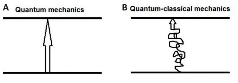
Figure 38. Schemes of Planck Quantum Transitions and Egorov Quantum-classical Transitions.

 

22.3 Nonlocal Phonons and Egorov Resonance

The natural vibrations of nuclei in molecules (local phonons) are a barrier to electronic transitions in them. This leads to broadening of optical bands[3,4]. Vibrations of nuclei in the medium (nonlocal phonons)[3] surrounding the molecules, as a rule, also lead to broadening of bands. However, there are exceptions to this rule, for example, polymethine dyes and their J-aggregates. Under the conditions of Egorov nano-resonance (see Equations (29-31)), nonlocal phonons are not a barrier to electronic transitions in them, but on the contrary, facilitate them. This is due to the quasilinear geometry of their extended π-electron optical chromophores (see Figures 9 and 12). The number of nonlocal phonons of the medium that effectively interact with the π-electron transition significantly exceeds the number of such local phonons in the chromophores themselves (see Sections 11 and 12). Under resonance conditions, the regular component of the reorganization motion of nonlocal phonons turns out to be coherent with the regular component of the π-electron motion and prevails over the chaotic components of both.

 

Note that the Egorov resonance condition

 

$$ \frac{EL}{\sqrt{J/2m}}=\hslash \left(101\right)$$

 

(see Equations (29-31)) can be interpreted in accordance with the Heisenberg uncertainty relation ΔpΔx=ℏ, where and Δx=L[15-17,38,117]. Unlike the Heisenberg uncertainty relation, in which Δp refers to a single quantum microparticle, such as an electron, the nuclear reorganization energy

 

$$ E=\frac{1}{2}{\sum }_{\kappa }\hslash {\omega }_{\kappa }{\stackrel{~}{q}}_{\kappa }^{2}$$

 

(see Equation (44)), included in Δp, contains an infinite number of vibrational modes κ of the environment. In addition, condition (101) is only a necessary condition for the Egorov resonance. The necessary and sufficient conditions for observing the Egorov resonance are condition (101) and the condition γ<<E, where γ is the dozy-chaos energy , see the caption to Figure 11).

 

22.4 J-band as a Signature of Polymethine Dyes

One may ask why the Egorov resonance is observed only in polymethine dyes and their J-aggregates. This is explained by the fact that the motion of the reorganization of the vibrations of the nuclei of the medium (methanol in the case of monomers of polymethine dyes and water in the case of J-aggregates) turns out to be coherent with the motion of the electron charge in the optical chromophore when this chromophore is a quasi-linear formation (Section 22.3). In the case of monomers, this is a quasi-one-dimensional polymethine chain along which the electron charge transfer occurs (Section 11, Figure 9). In the case of J-aggregates, this is a quasi-linear optical chromophore of four molecules in which the interaction of the π-electron transfer in the polymethine chain with the environment is enhanced by the addition of the π-system of the quasi-planar benzene rings of neighboring molecules (Section 12, Figures 11 and 12). I am not aware of any cases of observation of Egorov resonance in other molecules and/or molecular systems other than polymethines.

 

The fact of J-aggregation of polymethine dyes only in water and not in any other solvents has not yet been explained within the framework of theoretical methods of quantum chemistry.

 

22.5 The Singular Nature of the Franck‒Condon Principle and the Nature of the Physical Source of Life

On the path of consistent application of the Franck‒Condon principle, we arrive at a singular physical picture of molecular quantum transitions. Indeed, according to the Born‒Oppenheimer equations for the adiabatic approximation (see Equations (38) and (39))

 

$$ \left[\stackrel{\wedge }{{T}_{e}}+V\left(r,q\right)\right]{\psi }_{f}={U}_{f}\left(q\right){\psi }_{f}$$

 

$$ \left[\stackrel{\wedge }{{T}_{N}}+{U}_{f}\left(q\right)\right]{\varphi }_{fn}={E}_{fn}{\varphi }_{fn}$$

 

and according to the Franck‒Condon principle, with such a rapid vertical transition of an electron to another state, in which the nuclei do not have time to shift significantly, the entire electron‒nuclear system (for example, a molecule) ends up on the electronic term Uf(q). However, this term does not correspond to any stable state of the system until relaxation of the structure of the nuclear subsystem occurs, taking into account the new distribution of the electron charge. Such relaxation presupposes a “search” by nuclei for a new equilibrium position for their oscillations. Obviously, for this the nuclei must pass through the equilibrium position at least once in their oscillations. This circumstance gives an estimate for the resulting time of the entire electron transition, taking into account the relaxation of the nuclear subsystem, which is a value of the order of the half-period of the oscillations of the nuclei. However, this state of the entire system is not stable either, since the electron, as a result of the structural relaxation of the nuclei, is already in a new electric potential [V(r,q)]­1. Strictly speaking, the potential [V(r,q)]­1 differs from the potential V(r,q). Therefore, following the logic of the Born‒Oppenheimer adiabatic approximation and the Franck‒Condon principle, we must again solve the system of adiabatic Equations (38) and (39) and find a new electron term [Uf (q)]1. The structure of the oscillating nuclei must again relax to this new electron state, which also takes a time of the order of a half-period of their oscillations. As a result of this relaxation, the electron again finds itself in a certain new potential [V(r,q)]­2, which differs from the potential [V(r,q)]­1. And so on, until we obtain a self-consistent term [Uf (q)]∞ in an infinite time corresponding to an infinite number of half-periods of the oscillations of the nuclei.

 

Thus, by consistently applying the adiabatic approximation and the Franck‒Condon principle, we obtain a singular physical picture of molecular transitions. In this singular Franck‒Condon picture, the search for its new self-consistent molecular state occurs through the passage of an electron‒nuclear system through a huge (infinitely large) number of discrete steps of motion of both the electron and the nuclei over a huge (infinitely large) period of time. In Egorov’s QCM, this paradox, which exists in molecular quantum mechanics, is resolved due to chaotization, and therefore, the continuous nature of the dynamics of the transient molecular state. In Egorov’s mechanics, in the process of a molecular transition, an electron‒nuclear(‒oscillatory) system finds, due to the transient (dozy) chaos that entangles the electron and nuclear motions, its new self-consistent state not in a multi-stage, but in a single-stage dynamic picture and very quickly, in a time of the order of Planck’s constant divided by the energy of nuclear reorganization, which is a value of the order of femtoseconds.

 

I will note that my proof of the singularity of the Franck‒Condon principle does not require any graphic illustration. Moreover, such an illustration would be harmful to the proof itself. Any possible illustration would not correspond in reality to any physical mechanism of transitions of the entire molecular system between an enormous number of intermediate electron terms. In my proof, the only essential fact is that the Franck‒Condon principle, if we do not ignore the principle of causality, immediately leads to a multi-stage process of transitions of the electron‒nuclear system of the molecule between an infinite number of intermediate electron terms, a multi-stage process infinitely extended in time. In the standard interpretation of the Franck‒Condon principle, which is given in all textbooks, the principle of causality is ignored, and it is mistakenly assumed that the molecule passes to the final self-consistent term [Uf (q)]∞ immediately, that is, as a result of just one electron jump.

 

One of the main motivations for the further development of QCM is the fact that this new physical theory contains the source of dynamic and structural self-organization of molecular matter, up to the emergence of living matter[169]. The physical source of life is located in the gap between the energy levels of a valence electron in a molecule (see Figures 36 and 38B). The source of energy in this molecular “life machine” is the vibrations of nuclei, and the driver is valence electrons (see Sections 1 and 22.2). Dozy chaos in a complex physical system enables it to make a rational choice quickly and effectively. Without this kind of chaotic organization, no “life machine” can function.

 

Thus, standard quantum mechanics of molecules with its Franck‒Condon principle and without dozy chaos is an obstacle to finding out the nature of the physical source of life.

 

23 CONCLUSIONS

In this review, we compare two fundamentally different physical approaches to explaining the nature of the optical band shape of J-aggregates, the traditional approach based on the Frenkel exciton (Section 3) and the new approach based on QCM (Sections 5 and 6), and provide a reasoned choice between them in favor of the latter. In addition, we discuss the fundamentals of QCM as an alternative to quantum mechanics in molecular and chemical nanoscale physics (Sections 4 and 5).

 

In conventional molecular physics of small molecules, standard quantum mechanics can be used within the framework of the Born–Oppenheimer adiabatic approximation[2] and the Franck–Condon principle with its vertical electronic transitions (Sections 2 and 4)[7-10], since the shape of the optical spectra depends only on the characteristics of the initial and final states of the molecular transition and very weakly depend on the dynamics of the transient state[47], which, according to the new theory — QCM[11,15], is chaotic. In nanophysics, photochemistry and nanophotonics, where the spatial extent of a molecular transition can be large, that is, on the order of a nanometer or more, there is a need to take into account the regularity of the dynamics of the transient state, which occurs against the background of transient or dozy chaos[47].

 

In other words, since in the case of strong dozy chaos, which is almost always realized for sufficiently small molecules, the rates of QCTs do not depend on the specific dynamics of the transient state, but depend only on the initial and final states, we have the same result as in the standard Franck–Condon picture obtained within the framework of quantum mechanics[1]. Thus, we can obtain an explanation why the erroneous standard Franck–Condon picture[7-10] in the case of sufficiently small molecules is able to interpolate well experimental data[12-14] in standard molecular spectroscopy (Sections 2, 4 and 9). Note that a sophisticated researcher, especially a theoretical physicist, should not be confused by the conclusion that an erroneous theory and an erroneous physical picture can often be consistent with experimental data[47]. For example, the erroneous Aristotelian geocentric picture of the world has existed in human civilization for hundreds of years and is quite suitable from a practical point of view. If we discard the genius of Galileo and similar innovators, then the need for the emergence of a correct, namely heliocentric, picture of the world arose in practice only with the entry of mankind into space. A similar need arises in our time in the quantum physics of molecular physicochemical systems and in the quantum physics of condensed matter. Specifically, this need is expressed in the creation and development of QCM in all its comprehensiveness, which makes it possible to explain the chaotic and regular dynamics of the transient state in extended systems.

 

One of the most striking results of QCM is the resonance between electron motion and nuclear reorganization motion, called Egorov nano-resonance[15-20,49]. Egorov’s nano-resonance currently explains the nature of the well-known narrow and intense J-band of J-aggregates of polymethine dyes[15-20,49], which occurs in aqueous solutions of their monomers (Figures 11 and 12), as well as a resonance-like transformation of the shape of the optical bands of the dye monomer at different lengths of its polymethine chain (Figure 10).

 

In contrast to previous theories of the shape of optical bands of molecular aggregates, based on quantum mechanics and Frenkel’s exciton theory, the new theory, based on QCM and Egorov nano-resonance, allows us to explain not only the nature and shape of the J-band of J-aggregates, but also the nature and the shape of the polymethine dye monomer bands from which these J-aggregates are formed. This fact made it possible for the first time to theoretically explain all existing experimental shapes of optical bands of monomers (M) and J-aggregates in the well-known concentration equilibria in aqueous solutions of polymethine dyes, as well as to determine the number of molecules composing the optical J-chromophore, which is four (see Figures 11 and 12)[16,17,36-38].

 

Traditional ideas to explain the nature of the J-band of J-aggregates can be characterized as the emergence of a “vicious excitonic circle”, which began with the work of Franck and Teller[67], which explained the “red shift” by exciton selection rules in the “head-to-tail” configuration of monomers in the J-aggregate, as well as the work of Knapp[73], which explained the narrowing of the absorption band by averaging the statistical (static) disorder of the electronic energy levels of monomers in the J-aggregate by a fast-moving Frenkel exciton (Section 3.1). These and similar exciton concepts almost completely and unjustifiably dominate modern scientific consciousness and are associated not with scientific, but with psychological reasons.

 

Let us note the important role of the works of Petrenko & Stein[18,20], which, complementing the works of Egorov, together with them made it possible to break this “vicious excitonic circle”.

 

The theory of the narrow and intense J-band of J-aggregates is based on the discovery of QCM and Egorov’s nano-resonance in it. In QCM, chaos (dozy chaos) is a necessary condition for electron‒vibrational transitions. In other words, in real electron‒vibrational transitions there is always chaos. However, one electron, being very light, cannot “create” too much chaos. Therefore, the specific structure of the subsystem of very heavy nuclei interacting with a dynamically active electron during the transition plays an important role in the chaotic dynamics of the transition. Any spatially distinguished characteristic of the structure of the nuclear subsystem can introduce a significant regular component into the overall chaotic dynamics of the transition. Thus, in QCTs against the background of chaos, elements of dynamic organization (self-organization) arise. For example, in polymethine dyes, the basis of such dynamic self-organization is a quasi-linear and long polymethine chain, in which the π-electron charge transfer between carbon atoms occurs sequentially (Section 11, Figure 9). Experimentally, such self-organization is expressed in the resonant nature of the change in the shape of the optical absorption band with a change in the length of the polymethine chain, which determines the length of the QCT (Section 11, Figure 10). The transition from a one-dimensional structure to a two-dimensional brickwork-like structure due to J-aggregation through a two-dimensional π-system of benzene rings (Section 12, Figure 12) significantly enhances the dynamic self-organization due to a significant increase in the interaction of the π-electronic transition with vibrations of the surrounding nuclear subsystem. In other words, in quasi-two-dimensional J-aggregates with a brickwork-like structure under conditions of the nano-resonance against the background of general chaos, the regular component of the transition dynamics is much more pronounced than in quasi-linear monomers of polymethine dyes. This regular component of dynamics, like its chaotic component, is created in the process of reorganization of nuclear oscillations during electronic transitions.

 

Within the framework of QCM, an explanation is also given for the “red shift” of the nano-resonance in the monomer series of optical absorption bands depending on the decrease in the polarity of the solvent (Section 13).

 

Exciton theory and quantum-classical theory demonstrate fundamental differences in physical approaches to interpreting the nature of the narrow and intense J-band of J-aggregates (Section 19). In the exciton theory, the features of the optical spectrum of molecular monomers during J-aggregation are completely leveled out (Section 3.1), and in the quantum-classical theory, on the contrary, they are enhanced (Section 12). Namely, J-aggregation significantly enhances the Egorov nano-resonance, which is already observed in the vinylogous series of monomers (Section 11). In the experiment, the J-effect is manifested not by aggregates of any organic molecules, as is essentially assumed by the exciton approach, obtaining the J-band by simply enhancing the excitonic interaction in a linear chain of arbitrary molecules, but only by aggregates (J-aggregates, Section 12) of polymethine dye monomers having a specific optical chromophore (electron charge transfer chromophore, Section 11). Obviously, this fact speaks in favor of the quantum-classical approach rather than the excitonic one.

 

Based on QCM, an explanation is also given for the known shapes of optical bands of dimers, H- and H*-aggregates of polymethine dyes. An explanation is also given for the shapes of optical J-bands of absorption and luminescence of J-aggregates in Langmuir films and their anomalously small Stokes shift. A simple explanation is given for the detuning of the Egorov resonance in the well-known experiment of Hales et al.[133] upon the transition from one-photon to two-photon absorption of a selenopyrylium-terminated polymethine dye in chloroform, and experimental conditions for restoring the resonance shape of the optical band are predicted. Possible applications of QCM towards the creation of living materials and elucidation of the nature of the physical source of life are discussed.

 

Acknowledgements

This work was performed within the State assignment of NRC “Kurchatov Institute”.

 

Data Availability

This is a review paper and does not contain any original data. The data availability statements could be found in the original papers.

 

Copyright Permissions

Copyright © 2025 The Author(s). Published by Innovation Forever Publishing Group Limited. This open-access article is licensed under a Creative Commons Attribution 4.0 International License (https://creativecommons.org/licenses/by/4.0), which permits unrestricted use, sharing, adaptation, distribution, and reproduction in any medium, provided the original work is properly cited.

 

Conflicts of Interest

The author has no conflicts to disclose.

 

Author Contribution

All work for this review was done by Egorov VV.

 

Abbreviation List

QCM, Quantum-classical mechanics

QCT, Quantum-classical transition

QM, Quantum mechanics

TDPT, Time-dependent perturbation theory

 

References

[1] Davydov AS. Quantum Mechanics. Pergamon Press: Oxford, UK, 1976.

[2] Born M, Oppenheimer JR. On the quantum theory of molecules. Ann Phys-Berlin, 1927; 84: 457-484.[DOI]

[3] Perlin YE. Modern methods in the theory of many-phonon processes. Sov Phys Usp, 1964; 6: 542-565.[DOI]

[4] Frank-Kamenetskii MD, Lukashin AV. Electron–vibrational interactions in polyatomic molecules. Sov Phys Usp, 1975; 18: 391-409.[DOI]

[5] Bersuker IB, Polinger VZ. Vibronic Interactions in Molecules and Crystals. Springer: New York, NY, USA, 1989.[DOI]

[6] Stanke M. Adiabatic, Born–Oppenheimer, and Non-adiabatic Approaches. In: Leszczynski J, Kaczmarek-Kedziera A, Puzyn T et al (eds). Handbook of Computational Chemistry. Springer: Cham, Switzerland, 2017: 173-223.[DOI]

[7] Franck J, Dymond EG. Elementary processes of photochemical reactions. Trans Faraday Soc, 1925; 21: 536-542.[DOI]

[8] Condon EU. A theory of intensity distribution in band systems. Phys Rev, 1926; 28: 1182-1201.[DOI]

[9] Condon EU. Nuclear motions associated with electron transitions in diatomic molecules. Phys Rev, 1928; 32: 858-872.[DOI]

[10] Condon EU. The Franck–Condon principle and related topics. Am J Phys, 1947; 15: 365-374.[DOI]

[11] Egorov VV. Quantum–classical mechanics as an alternative to quantum mechanics in molecular and chemical physics. Heliyon, 2019; 5: e02579.[DOI]

[12] Herzberg G, Spinks JWT. Molecular Spectra and Molecular Structure. I. Spectra of Diatomic Molecules. Prentice-Hall: New York, NY, USA, 1939.

[13] Herzberg G. Molecular Spectra and Molecular Structure. II. Infrared and Raman Spectra of Polyatomic Molecules. D. Van Nostrand: New York, NY, USA, 1945.

[14] Herzberg G. Molecular Spectra and Molecular Structure. III. Electronic Spectra and Electronic Structure of Polyatomic Molecules. D. Van Nostrand: New York, NY, USA, 1966.

[15] Egorov VV. Quantum–classical mechanics: Nano-resonance in polymethine dyes. Mathematics, 2022; 10: 1443.[DOI]

[16] Egorov VV, Alfimov MV. Theory of the J-band: From the Frenkel exciton to charge transfer. Phys Usp, 2007; 50: 985-1029.[DOI]

[17] Egorov VV. Theory of the J-band: From the Frenkel exciton to charge transfer. Phys Procedia, 2009; 2: 223-326.[DOI]

[18] Petrenko A, Stein M. Toward a molecular reorganization energy-based analysis of third-order nonlinear optical properties of polymethine dyes and J-aggregates. J Phys Chem A, 2019; 123: 9321-9327.[DOI]

[19] Egorov VV, Thomas S. Quantum–classical mechanics: On the problem of a two-photon resonance band shape in polymethine dyes. Nano-Struct Nano-Objects, 2021; 25: 100650.[DOI]

[20] Petrenko A, Stein M. Molecular reorganization energy as a key determinant of J-band formation in J-aggregates of polymethine dyes. J Phys Chem A, 2015; 119: 6773-6780.[DOI]

[21] James TH. The Theory of the Photographic Process, 4th ed. Macmillan: New York, NY, USA, 1977.

[22] Herz AH. Aggregation of sensitizing dyes in solution and their adsorption onto silver halides. Adv Colloid Interface Sci, 1977; 8: 237-298.[DOI]

[23] Kobayashi T. J-Aggregates. World Scientific: Singapore, Singapore, 1996.

[24] Harrison WJ, Mateer DL, Tiddy GJT. Liquid-crystalline J-Aggregates formed by aqueous ionic cyanine dyes. J Phys Chem, 1996; 100: 2310-2321.[DOI]

[25] Würthner F, Kaiser TE, Saha-Möller CR. J-aggregates: From serendipitous discovery to supra-molecular engineering of functional dye materials. Angew Chem Int Edit, 2011; 50: 3376-3410.[DOI]

[26] Aviv H, Tischler YR. Synthesis and characterization of a J-aggregating TDBC derivative in solution and in Langmuir–Blodgett films. J Lumin, 2015; 158: 376-383.[DOI]

[27] Bricks JL, Slominskii YL, Panas ID, Demchenko AP. Fluorescent J-aggregates of cyanine dyes: Basic research and applications review. Methods Appl Fluoresc, 2018; 6: 012001.[DOI]

[28] Berlepsch H, Böttcher C. Tubular J-aggregates of a new thiacarbocyanine Cy5 dye for the far-red spectral region—a spectroscopic and cryo-transmission electron microscopy study. Phys Chem Chem Phys, 2018; 20: 18969-18977.[DOI]

[29] Jelley EE. Spectral absorption and fluorescence of dyes in the molecular state. Nature, 1936; 138: 1009-1010.[DOI]

[30] Jelley EE. Molecular, nematic and crystal states of 1:1′-diethyl-ψ-cyanine chloride. Nature, 1937; 139: 631-632.[DOI]

[31] Scheibe G. Variability of the absorption spectra of some sensitizing dyes and its cause. Angew Chem, 1936; 49: 563-564.

[32] Scheibe G. On the variability of the absorption spectra in solutions and the secondary bonds as its cause. Angew Chem, 1937; 50: 212-219.[DOI]

[33] Egorov VV. Quantum–classical mechanics: Luminescence spectra in polymethine dyes and J-aggregates. Nature of the small Stokes shift. Res Phys, 2019; 13: 102252.[DOI]

[34] Egorov VV. Nature of the optical band shapes in polymethine dyes and H-aggregates: Dozy chaos and excitons. Comparison with dimers, H- and J-aggregates. R Soc Open Sci, 2017; 4: 160550.[DOI]

[35] Egorov VV. Optical lineshapes for dimers of polymethine dyes: Dozy-chaos theory of quantum transitions and Frenkel exciton effect. RSC Adv, 2013; 3: 4598-4609.[DOI]

[36] Egorov VV. Electron-transfer approach to the nature of the optical lineshape for molecular J-aggregates. Chem Phys Lett, 2001; 336: 284-291.[DOI]

[37] Egorov VV. On electrodynamics of extended multiphonon transitions and nature of the J-band. Chem Phys, 2001; 269: 251-283.[DOI]

[38] Egorov VV. Nature of the optical transition in polymethine dyes and J-aggregates. J Chem Phys, 2002; 116: 3090-3103.[DOI]

[39] Egorov VV. Discovery of Dozy Chaos and Discovery of Quanta: Analogy Being in Science and Perhaps in Human Progress. In: Stavrinides SG, Banerjee S, Caglar H et al (eds). Chaos and Complex Systems. Proceedings of the 4th International Interdisciplinary Chaos Symposium. Springer: Berlin, Germany, 2013: 41-46.[DOI]

[40] Egorov VV. Dozy Chaos in Chemistry: Simplicity in Complexity. In: Stavrinides SG, Banerjee S, Caglar H et al (eds). Chaos and Complex Systems. Proceedings of the 4th International Interdisciplinary Chaos Symposium. Springer: Berlin, Germany, 2013: 219-224.[DOI]

[41] Egorov VV. Dozy-chaos mechanics for a broad audience. Challenges, 2020; 11: 16.[DOI]

[42] Dirac PAM. The quantum theory of the emission and absorption of radiation. Proc R Soc Lond A Math Phys Sci, 1927; 114: 243-265.[DOI]

[43] Fermi E. Quantum theory of radiation. Rev Mod Phys, 1932; 4: 87-132.[DOI]

[44] Berestetskii VB, Lifshitz EM, Pitaevskii LP. Quantum Electrodynamics, 2nd ed. Elsevier: Amsterdam, Netherlands, 1982.

[45] Landau LD, Lifshitz EM. Quantum Mechanics, Non-Relativistic Theory, 3rd ed. Elsevier: Amsterdam, Netherlands, 1977.

[46] Planck M. On the law of distribution of energy in the normal spectrum. Ann Phys-Berlin, 1901; 4: 553-563.[DOI]

[47] Egorov VV. Quantum–classical mechanics and the Franck–Condon principle. Comput Sci Math Forum, 2023; 7: 55.[DOI]

[48] Scholes GD, Fleming GR, Chen LX et al. Using coherence to enhance function in chemical and biophysical systems. Nature, 2017; 543: 647-656.[DOI]

[49] Egorov VV. The J-band of J-aggregates as the Egorov nano-resonance. Comput Sci Math Forum, 2023; 7: 31.[DOI]

[50] Ghose P. A continuous transition between quantum and classical mechanics. Found Phys, 2002; 32: 871-892.[DOI]

[51] Ghose P, Samal MK. A continuous transition between quantum and classical mechanics. II. Found Phys, 2002; 32: 893-906.[DOI]

[52] Billing GD. Quantum-dressed classical mechanics: Theory and application. Phys Chem Chem Phys, 2002; 4: 2865-2877.[DOI]

[53] Tully JC. Mixed quantum–classical dynamics. Faraday Discuss, 1998; 110: 407-419.[DOI]

[54] Bultrini D, Vendrell O. Mixed quantum‒classical dynamics for near term quantum computers. Commun Phys, 2023; 6: 328.[DOI]

[55] Schrödinger E. Quantisierung als eigenwertproblem. Ann Phys, 1926; 79: 361-376.[DOI]

[56] Heitler W. The Quantum Theory of Radiation, 3rd ed. Clarendon Press: Oxford, UK, 1954.

[57] Baz’ AI, Zel’dovich YB, Perelomov AM. Scattering, Reactions, and Decays in Nonrelativistic Quantum Mechanics, 2nd ed. Nauka: Moscow, Russia, 1971.

[58] Deshmukh AP, Geue N, Bradbury NC et al. Bridging the gap between H- and J-aggregates: Classification and supramolecular tunability for excitonic band structures in two-dimensional molecular aggregates. Chem Phys Rev, 2022; 3: 021401.[DOI]

[59] Kubo R. A stochastic theory of line shape. Adv Chem Phys, 1969; 15: 101-127.[DOI]

[60] Egorov VV. Dynamic pumping of elementary charge transfer by environmental dissipative reorganization. Russ J Electrochem, 2003; 39: 86-96.[DOI]

[61] Scherer POJ. Molecular Aggregate Spectra. In: Kobayashi T (ed). J-Aggregates. World Scientific: Singapore, 1996: 95-110.[DOI]

[62] Davydov AS. Theory of Molecular Excitons. McGraw-Hill: New York, USA, 1962.

[63] Knox RS. Theory of Excitons. Academic Press: New York, USA, 1963.

[64] Agranovich VM. The Theory of Excitons. Nauka: Moscow, Russia, 1968.

[65] Frenkel J. On the transformation of light into heat in solids.  Phys Rev, 1931; 37: 17-44, 1276-1294.[DOI]

[66] Knoester J, Spano FC. Theory of Pump-Probe Spectroscopy of Molecular J-Aggregates. In: Kobayashi T (ed). J-Aggregates. World Scientific: Singapore, 1996: 111-161.[DOI]

[67] Franck J, Teller E. Migration and photochemical action of excitation energy in crystals. J Chem Phys, 1938; 6: 861-872.[DOI]

[68] McRae EG, Kasha M. Enhancement of phosphorescence ability upon aggregation of dye molecules. J Chem Phys, 1958; 28: 721-722.[DOI]

[69] Kasha M. Relation between exciton bands and conduction bands in molecular lamellar systems. Rev Mod Phys, 1959; 31: 162-169.[DOI]

[70] Kasha M. Energy transfer mechanisms and the molecular exciton model for molecular aggregates. Radiat Res, 1963; 20: 55-70.[DOI]

[71] McRae EG, Kasha M. The Molecular Exciton Model. In: Augenstein L, Mason R, Rosenberg B (eds). Physical Processes in Radiation Biology. Academic Press: New York, USA, 1964: 23-42.[DOI]

[72] Kasha M, Rawls HR, El-Bayoumi MA. The exciton model in molecular spectroscopy. Pure Appl Chem, 1965; 11: 371-392.[DOI]

[73] Knapp EW. Lineshapes of molecular aggregates. Exchange narrowing and intersite correlation. Chem Phys, 1984; 85: 73-82.[DOI]

[74] Knapp EW, Scherer POJ, Fischer SF. On the lineshapes of vibronically resolved molecular aggregate spectra. Chem Phys Lett, 1984; 111: 481-486.[DOI]

[75] Makhov DV, Egorov VV, Bagatur’yants AA et al. Numerical calculations of optical lineshapes for disordered molecular aggregates. Chem Phys Lett, 1995; 246: 371-380.[DOI]

[76] Makhov DV, Egorov VV, Bagatur’yants AA et al. Calculations of the optical line shapes for disordered molecular aggregates using the resolvent of the Hamiltonian. J Lumin, 1997; 72-74: 439-441.[DOI]

[77] Makhov DV, Egorov VV, Bagatur’yants AA et al. Calculations of the optical lineshapes for disordered molecular aggregates: Effects of aggregate structure. Mater Sci Eng C, 1998; 5: 311-315.[DOI]

[78] Makhov DV, Egorov VV, Bagatur’yants AA et al. Efficient approach to the numerical calculation of optical line shapes for molecular aggregates. J Chem Phys, 1999; 110: 3196-3199.[DOI]

[79] Bakalis LD, Knoester J. Pump−probe spectroscopy and the exciton delocalization length in molecular aggregates. J Phys Chem B, 1999; 103: 6620-6628.[DOI]

[80] Eisfeld A, Briggs JS. The J-band of organic dyes: Lineshape and coherence length. Chem Phys, 2002; 281: 61-70.[DOI]

[81] Bednarz M, Malyshev VA, Knoester J. Low-temperature dynamics of weakly localized Frenkel excitons in disordered linear chains. J Chem Phys, 2004; 120: 3827-3840.[DOI]

[82] Spano FC. The spectral signatures of Frenkel polarons in H- and J-aggregates. Acc Chem Res, 2010; 43: 429-439.[DOI]

[83] Hestand NJ, Spano FC. Expanded theory of H- and J-molecular aggregates: The effects of vibronic coupling and intermolecular charge transfer. Chem Rev, 2018; 118: 7069-7163.[DOI]

[84] Fidder H, Terpstra J, Wiersma DA. Dynamics of Frenkel excitons in disordered molecular aggregates. J Chem Phys, 1991; 94: 6895-6907.[DOI]

[85] Fidder H, Knoester J, Wiersma DA. Optical properties of disordered molecular aggregates: A numerical study. J Chem Phys, 1991; 95: 7880-7890.[DOI]

[86] Briggs JS, Herzenberg A. Bandshapes in polymer spectra. Mol Phys, 1971; 21: 865-879.[DOI]

[87] Wubs M, Knoester J. Exchange narrowing in dynamically disordered molecular aggregates. Chem Phys Lett, 1998; 284: 63-70.[DOI]

[88] Malyshev VA. Localization length of one-dimensional exciton and low-temperature behaviour of radiative lifetime of J-aggregated dye solutions. J Lumin, 1993; 55: 225-230.[DOI]

[89] Mukamel S. Principles of Nonlinear Optical Spectroscopy. Oxford University Press: New York, 1995.

[90] Argyrakis P, Basco DM, Drobizhev MA et al. Absorption lineshape of J-aggregates of thiacarbocyanine dyes: Experiment and numerical study. Chem Phys Lett, 1997; 268: 372-380.[DOI]

[91] Kuhn H, Kuhn C. Chromophore Coupling Effects. In: Kobayashi T (ed). J-Aggregates. World Scientific, Singapore, 1996: 1-40.[DOI]

[92] Dähne S. Color and constitution: One hundred years of research. Science, 1978; 199: 1163-1167.[DOI]

[93] Kachkovskii AD. The nature of electronic transitions in linear conjugated systems. Russ Chem Rev, 1997; 66: 647-664.[DOI]

[94] Burshtein KY, Bagatur’yants AA, Alfimov MV. MO calculations on the absorption spectra of organic dimers. Chem Phys Lett, 1995; 239: 195-200.[DOI]

[95] Sevian HM, Skinner JL. Molecular theory of transition energy correlations for pairs of chromophores in liquids or glasses. J Chem Phys, 1992; 97: 8-18.[DOI]

[96] Van Burgel M, Wiersma DA, Duppen K. The dynamics of one-dimensional excitons in liquids. J Chem Phys, 1995; 102: 20-33.[DOI]

[97] Durrant JR, Knoester J, Wiersma DA. Local energetic disorder in molecular aggregates probed by the one-exciton to two-exciton transition. Chem Phys Lett, 1994; 222: 450-456.[DOI]

[98] Knoester J. Nonlinear optical line shapes of disordered molecular aggregates: Motional narrowing and the effect of intersite correlations. J Chem Phys, 1993; 99: 8466-8479.[DOI]

[99] Moll J, Dähne S, Durrant JR et al. Optical dynamics of excitons in aggregates of a carbocyanine dye. J Chem Phys, 1995; 102: 6362-6370.[DOI]

[100] Malyshev VA, Rodríguez A, Domínguez-Adame F et al. Linear optical properties of one-dimensional Frenkel exciton systems with intersite energy correlations. Phys Rev B, 1999; 60: 14140-14146.[DOI]

[101] Guerrini M, Calzolari A, Varsano D et al. Quantifying the plasmonic character of optical excitations in a molecular J-aggregate. J Chem Theory Comput, 2019; 15: 3197-3203.[DOI]

[102] Egorov VV. Optical line shapes for polymethine dyes and their aggregates: Novel theory of quantum transitions and its correlation with experiment. J Lumin, 2011; 131: 543-547.[DOI]

[103] Egorov VV. Nature of the narrow optical band in H*-aggregates: Dozy-chaos–exciton coupling. AIP Adv, 2014; 4: 077111.[DOI]

[104] Qian Y, Li X, Harutyunyan AR et al. Herzberg–Teller effect on the vibrationally resolved absorption spectra of single-crystalline pentacene at finite temperatures. J Phys Chem A, 2020; 124: 9156‒9165.[DOI]

[105] Mustroph H. Potential-energy surfaces, the Born–Oppenheimer approximations, and the Franck–Condon principle: Back to the roots. Chem Phys Chem, 2016; 17: 2616-2629.[DOI]

[106] Huang K, Rhys A. Theory of light absorption and non-radiative transitions in F-centres. Proc R Soc A, 1950; 204: 406-423.[DOI]

[107] Feynman RP. An operator calculus having applications in quantum electrodynamics. Phys Rev, 1951; 84: 108-128.[DOI]

[108] Lax M. The Franck‒Condon principle and its application to crystals. J Chem Phys, 1952; 20: 1752-1760.[DOI]

[109] Krivoglaz MA, Pekar SI. The shape of the spectra of the impurity light absorption and luminescence in dielectrics [In Russian]. Tr Inst Fiz Akad Nauk Ukr SSR, 1953; 4: 37-70.

[110] Krivoglaz MA. The theory of thermal transitions [In Russian]. Zh Eksp Teor Fiz, 1953; 25: 191-207.

[111] Kubo R, Toyozawa Y. Application of the method of generating function to radiative and non-radiative transitions of a trapped electron in a crystal. Prog Theor Phys, 1955; 13: 160-182.[DOI]

[112] Schrödinger E. Statistical Thermodynamics. Cambridge University Press: Cambridge, UK, 1946.

[113] Egorov VV. Theory of tunnel transfer. Khim Fiz, 1988; 7: 1466-1482 Sov J Chem Phys, 1991; 7: 2629-2660.

[114] Sil’d O. Zero-Phonon Lines and Spectral Hole Burning in Spectroscopy and Photochemistry. Springer-Verlag: Berlin, Germany, 1988.

[115] Abramowitz M, Stegun IA. Handbook of Mathematical Functions. Dover Publications: New York, USA, 1965.

[116] Pekar SI. Theory of F-centers [In Russian]. Zh Eksp Teor Fiz, 1950; 20: 510-522.

[117] Egorov VV. Dynamic Symmetry in Dozy-Chaos Mechanics. In: Volos C. Symmetry in Chaotic Systems and Circuits. MDPI: Basel, Switzerland, 2022: 199-217.[DOI]

[118] Marcus RA. On the theory of oxidation-reduction reactions involving electron transfer. J Chem Phys, 1956; 24: 867-978.[DOI]

[119] Marcus RA, Sutin N. Electron transfers in chemistry and biology. Biochim Biophys Acta, 1985; 811: 265-322.[DOI]

[120] Marcus RA. Electron transfer reactions in chemistry. Theory and experiment. Rev Mod Phys, 1993; 65: 599-610.[DOI]

[121] Pekar SI. To the theory of luminescence and light absorption by impurities in dielectrics [In Russian]. Zh Eksp Teor Fiz, 1952; 22: 641-657.

[122] Pekar SI. On the effect of lattice deformations by electrons on optical and electrical properties of crystals [In Russian]. Uspekhi Fiz Nauk, 1953; 50: 197-252.[DOI]

[123] Brooker LGS, Sprague RH, Smith CP et al. Color and constitution. I. Halochromism of anhydronium bases related to the cyanine dyes. J Am Chem Soc, 1940; 62: 1116-1125.[DOI]

[124] Zhao YS, Fu H, Peng A et al. Construction and optoelectronic properties of organic one-dimensional nanostructures. Acc Chem Res, 2010; 43: 409-418.[DOI]

[125] Hunter CA, Sanders JKM. The nature of pi‒pi interactions. J Am Chem Soc, 1990; 112: 5525-5534.[DOI]

[126] McGaughey GB, Gagné M, Rappé AK. pi-Stacking interactions. Alive and well in proteins. J Biol Chem, 1998; 273: 15458-15463.[DOI]

[127] Bloom JWG, Wheeler SE. Taking the aromaticity out of aromatic interactions. Angew Chem Int Ed, 2011; 50: 7847-7849.[DOI]

[128] Martinez CR, Iverson BL. Rethinking the term “pi-stacking”. Chem Sci, 2012; 3: 2191-2201.[DOI]

[129] Wheeler SE, Bloom JWG. Toward a more complete understanding of noncovalent interactions involving aromatic rings. J Phys Chem A, 2014; 118: 6133-6147.[DOI]

[130] Avakyan VG, Shapiro BI, Alfimov MV. Dimers, tetramers, and octamers of mono- and trimethyne thiacarbocyanine dyes. Dyes Pigm, 2014; 109: 21-33.[DOI]

[131] Wheeler SE. Unraveling the Origin of Substituents Effects in π-Stacking Interactions. In: Scheiner S (ed). Noncovalent Forces. Springer: Cham, Switzerland, 2015: 421-442.[DOI]

[132] Kachkovski OD, Tolmachov OI, Slominskii YL et al. Electronic properties of polymethine systems 7: Soliton symmetry breaking and spectral features of dyes with a long polymethine chain. Dyes Pigm, 2005; 64: 207-216.[DOI]

[133] Hales JM, Matichak J, Barlow S et al. Design of polymethine dyes with large third-order optical nonlinearities and loss figures of merit. Science, 2010; 327: 1485-1488.[DOI]

[134] Didraga C, Pugžlys A, Hania PR et al. Structure, spectroscopy, and microscopic model of tubular carbocyanine dye aggregates. J Phys Chem B, 2004; 108: 14976‒14985.[DOI]

[135] Gurevich YY, Pleskov YV. New problems and prospects in the electrochemistry of semiconductors. Russ Chem Rev, 1983; 52: 318-336.[DOI]

[136] Shapiro BI. Aggregates of cyanine dyes: Photographic problems. Russ Chem Rev, 1994; 63: 231-255.[DOI]

[137] Lenhard JR, Hein BR. Effects of J-aggregation on the redox levels of a cyanine dye. J Phys Chem, 1996; 100: 17287‒17296.[DOI]

[138] Shapiro BI. Molecular assemblies of polymethine dyes. Russ Chem Rev, 2006; 75: 433-456.[DOI]

[139] Egorov VV. Quantum-classical mechanics as a guide to finding the simplest form of life organization and looking beyond the horizon. Sci Academique, 2023; 4: 7-11.

[140] Vitas M, Dobovišek A. A possible origin of life in nonpolar environments. BioSystems, 2025; 247: 105384.[DOI]

[141] Pace NR. The universal nature of biochemistry. PNAS, 2001; 98: 805-808.[DOI]

[142] Bains W. Many chemistries could be used to build living systems. Astrobiology, 2004; 4: 137-167.[DOI]

[143] Davies PCW, Lineweaver CH. Finding a second sample of life on Earth. Astrobiology, 2005; 5: 154-163.[DOI]

[144] Cleland CE, Copley SD. The possibility of alternative microbial life on Earth. Int J Astrobiology, 2006; 4: 165‒173.[DOI]

[145] Davies PCW, Benner SA, Cleland CE et al. Signatures of a shadow biosphere. Astrobiology, 2009; 9: 241-249.[DOI]

[146] Benner SA. Defining life. Astrobiology, 2010; 10: 1021-1030.[DOI]

[147] Des Marais DJ, Nuth III JA, Allamandola LJ et al. The NASA astrobiology roadmap. Astrobiology, 2008; 8: 715-730.[DOI]

[148] Davila AF, McKay CP. Chance and necessity in biochemistry: Implications for the search for extraterrestrial biomarkers in Earth-like environments. Astrobiology, 2014; 14: 534‒540.[DOI]

[149] Qian GR, Niu H, Hu CH et al. Diverse chemistry of stable hydronitrogens, and implications for planetary and materials sciences. Sci Rep, 2016; 6: 25947.[DOI]

[150] Stevenson J, Lunine J, Clancy P. Membrane alternatives in worlds without oxygen: Creation of an azotosome. Sci Adv, 2015; 1: e1400067.[DOI]

[151] Palmer MY, Cordiner MA, Nixon CA et al. ALMA detection and astrobiological potential of vinyl cyanide on Titan. Sci Adv, 2017; 3: e1700022.[DOI]

[152] Sandström H, Rahm M. Can polarity-inverted membranes self-assemble on Titan? Sci Adv, 2020; 6: eaax0272.[DOI]

[153] Hoshika S, Leal NA, Kim MJ et al. Hachimoji DNA and RNA: A genetic system with eight building blocks. Science, 2019; 363: 884-887.[DOI]

[154] Tsytovich VN, Morfill GE, Fortov VE et al. From plasma crystals and helical structures towards inorganic living matter. New J Phys, 2007; 9: 263.[DOI]

[155] Anchordoqui LA, Chudnovsky EM. Can self-replicating species flourish in the interior of a star? Lett High Energy Phys, 2020; 166: 1-4.[DOI]

[156] Jansen TLC, Günther LM, Knoester J et al. Electronically excited states in cylindrical molecular aggregates: Exciton delocalization, dynamics, and optical response. Chem Phys Rev, 2024; 5: 041305.[DOI]

[157] Zhong K, Nguyen HL, Do TN et al. Coarse-grained approach to simulate signatures of excitation energy transfer in two-dimensional electronic spectroscopy of large molecular systems. J Chem Theory Comput, 2024; 20: 6111-6124.[DOI]

[158] Erić V, Castro JL, Li X et al. Ultrafast anisotropy decay reveals structure and energy transfer in supramolecular aggregates. J Phys Chem B, 2023; 127: 7487‒7496.[DOI]

[159] Manrho M, Krishnaswamy SR, Kriete B et al. Watching molecular nanotubes self-assemble in real time. J Am Chem Soc, 2023; 145: 22494-22503.[DOI]

[160] Prokhorov VV, Prusakov KA, Pozin SI et al. Crystallographic models of ribbons and ribbon-based J-aggregate nanotubes from the geometry of tube ends. Phys Chem Chem Phys, 2024; 26: 28650-28661.[DOI]

[161] Erić V, Li X, Dsouza L et al. Manifestation of hydrogen bonding and exciton delocalization on the absorption and two-dimensional electronic spectra of chlorosomes. J Phys Chem B, 2023; 127: 1097-1109.[DOI]

[162] Frehan SK, Dsouza L, Li X et al. Photon energy-dependent ultrafast exciton transfer in chlorosomes of Chlorobium tepidum and the role of supramolecular dynamics. J Phys Chem B, 2023; 127: 7581-7589.[DOI]

[163] Dsouza L, Li X, Erić V et al. An integrated approach towards extracting structural characteristics of chlorosomes from a bchQ mutant of Chlorobaculum tepidum. Phys Chem Chem Phys, 2024; 26: 15856-5867.[DOI]

[164] Erić V, Li X, Dsouza L et al. Observation of dark states in two-dimensional electronic spectra of chlorosomes. J Phys Chem B, 2024; 128: 3575-3584.[DOI]

[165] Zhong K, Erić V, Nguyen HL et al. Application of the time-domain multichromophoric fluorescence resonant energy transfer method in the NISE programme. J Chem Theory Comput, 2025; 21: 254-266.[DOI]

[166] Nakakuki K, Sasaki SI, Tamiaki H. Self-aggregation of synthetic 7- or 8-unsubstituted bacteriochlorophyll-d analogs. J Photoch Photobio A, 2025; 462: 116257.[DOI]

[167] Manrho M, Jansen TLC, Knoester J. Optical signatures of the coupling between excitons and charge transfer states in linear molecular aggregates. J Chem Phys, 2022; 156: 224112.[DOI]

[168] Jansen TLC. Computational spectroscopy of complex systems. J Chem Phys, 2021; 155: 170901.[DOI]

[169] Quantum theory: From Planck to Egorov. American Association for the Advancement of Science (AAAS) press-release. Accessed 22 January 2025. Available at:[Web]