Enhanced Predictive Ensemble Learning Models for Compressive Strength of Concrete Modified with Bentonite Clay

 

Amir Tavana Amlashi1*, Ali Reza Ghanizadeh2, Samer Dessouky1

 

1School of Civil and Environmental Engineering and Construction Management, University of Texas at San Antonio, San Antonio, Texas, USA

2Department of Civil Engineering, Sirjan University of Technology, Sirjan, Iran

 

*Correspondence to: Amir Tavana Amlashi, School of Civil and Environmental Engineering and Construction Management, University of Texas at San Antonio, San Antonio, Texas, 78282, USA; Email: Amir.tavanaamlashi@my.utsa.edu

 

DOI: 10.53964/id.2024033

 

Abstract

This study addresses the logistical challenges of testing bentonite plastic concrete in the field by developing predictive models for compressive strength (CS) using Python-based machine learning techniques. The models, including random forest, adaptive boosting, extreme gradient boosting, and gradient boosting regression tree, were enhanced with forensic-based investigation optimization. A dataset of 285 CS records was used to train and validate these models. SHAP analysis highlighted the impact of various inputs like gravel, bentonite, curing time, and cement on CS. Results show that the GBRT-FBIO model outperformed the others in CS prediction, indicating its superior effectiveness for material science applications.

 

Keywords: bentonite plastic concrete, random forest, adaptive boosting, extreme gradient boosting, gradient boosting regression tree, shap analysis, forensic-based investigation optimization

 

1 INTRODUCTION

Waste management is a critical global challenge as industries and societies push toward sustainability. One of the key issues in this domain is heavy metal contamination in wastewater which arises from various industrial processes, including mining, electroplating, and metal refining[1]. Heavy metals such as chromium (Cr), mercury (Hg), copper (Cu), lead (Pb), cadmium (Cd), zinc (Zn), and nickel (Ni) pose significant ecological hazards because they do not degrade and tend to bioaccumulate in organisms, causing severe health and environmental issues[2,3].Traditional methods for treating wastewater, such as chemical precipitation and ion exchange, can be costly and sometimes ineffective at removing trace levels of heavy metals. Adsorption, especially using clay minerals, has emerged as an efficient and economical method for removing these pollutants[4].

 

Bentonite, a clay composed primarily of montmorillonite, has proven to be particularly effective for heavy metal adsorption due to its large surface area, high cation exchange capacity, low cost, and non-toxic nature[5,6]. Several studies have demonstrated the potential of bentonite for removing heavy metals from water[7,8]. The combination of bentonite with concrete, forming what is known as bentonite plastic concrete (BPC), enhances the material’s properties for environmental engineering applications. Specifically, BPC is valued for its low permeability, which makes it ideal for use in structures like dam cutoff walls to prevent water seepage[9]. Research has shown that BPC can absorb water and expand, contributing to its effective performance in limiting seepage and increasing the longevity of engineering structures[10].

 

BPC has seen widespread use in projects where controlling seepage is crucial, such as dam construction, where it reduces the risk of structural failure caused by internal water pressure and soil movement[11]. Despite its advantages, the preparation, testing, and optimization of BPC mixtures are labor-intensive and costly, often requiring specialized equipment and skilled personnel. These factors drive the need for computational models that can predict the material’s behavior, particularly its compressive strength (CS), without relying on extensive physical testing[12].

 

Recent advances in machine learning (ML) and artificial intelligence (AI) have opened up new possibilities for material property prediction. ML techniques such as artificial neural networks (ANN), support vector machines (SVM), and ensemble learning methods like gradient boosting regression tree (GBRT) and random forest (RF) have demonstrated superior accuracy in predicting concrete properties compared to traditional regression-based methods[13-15]. These methods can model complex, non-linear relationships between input variables, providing precise predictions without requiring large-scale experimental data[16,17]. For BPC, previous studies have applied various ML techniques to predict key properties such as slump, elastic modulus, and CS. For instance, Tavana Amlashi et al.[18] found that ANN models were more accurate than conventional methods for predicting the mechanical properties of BPC, while Ghanizadeh et al.[14] demonstrated that SVM and ANN could effectively predict CS, with cement content and silty clay showing the greatest and least influence, respectively, on the material’s performance.

 

In more recent work, hybrid AI models, such as Adaptive Neuro-Fuzzy Inference Systems (ANFIS) optimized with Particle Swarm Optimization, have been shown to outperform standalone models, achieving high accuracy in predicting the CS and tensile strength of plastic concretes[19]. Similarly, other computational techniques, including response surface methodology (RSM), multigene genetic programming (MGGP), and the group method of data handling (GMDH), have also been employed to model the mechanical properties of BPC using input parameters such as water content, bentonite, cement, sand, gravel, and curing time[20]. Ensemble learning models, which combine the predictions of multiple base learners to improve performance, are particularly promising for this task. Algorithms such as GBRT, extreme gradient boosting (XGB), and RF have shown notable success in predicting the mechanical properties of various concrete types, including high-performance concrete (HPC), recycled aggregate concrete (RAC), and geopolymer concrete (GPC)[21,22].

 

One of the limitations in existing studies is the lack of robustness in these ML models when applied to diverse datasets, as well as insufficient attention to meta-parameter optimization, which is crucial for improving model performance[23]. Tuning meta-parameters in ensemble learning (EL) models, including the number of estimators, learning rate, and tree depth, can significantly impact the accuracy and generalizability of predictions. Recognizing this gap, recent work has proposed various metaheuristic optimization techniques to address the challenges of manual parameter selection[24,25]. Among these, the forensic-based investigation optimization (FBIO) algorithm has emerged as an effective tool for fine-tuning the meta-parameters of ML models, ensuring that ensemble methods such as boosting and bagging achieve their full predictive potential[26]. FBIO mimics the process of forensic investigations, iteratively narrowing down the search space to find optimal solutions, thus improving model accuracy while reducing the computational effort required for parameter tuning[27].

 

This study seeks to fill the gaps in current research by developing a robust ensemble learning framework, integrated with FBIO, to predict the compressive strength of BPC. By utilizing a comprehensive dataset of 285 CS test records and employing advanced machine learning techniques such as RF, ADB, GBRT, and XGB, this research aims to provide more accurate and generalizable models for BPC strength prediction. Additionally, SHapley Additive exPlanations (SHAP) are used to interpret the influence of input variables on model predictions, ensuring transparency and interpretability of the results. This approach offers a significant improvement over existing methods by reducing the reliance on costly experimental testing while enhancing the understanding of how various factors-such as gravel content, curing time, and cement-affect BPC’s performance.

 

2 METHODOLOGY

This study employs several advanced machine learning algorithms to predict the compressive strength of BPC. ADB, introduced by Schapire[28], is a boosting method that combines weak learners iteratively, improving model accuracy over time by focusing on misclassified samples[29]. Decision trees (DT) and ANN are commonly used within this framework due to their versatility in handling both regression and classification tasks[30,31]. GBRT, based on the classification and regression tree (CART) method[32], improves predictions by incorporating poor learners in each iteration, reducing forecasting errors[33]. This technique is highly effective in improving the accuracy of weak learners, particularly in regression applications, making it a suitable candidate for predicting the compressive strength of BPC. XGB, developed by Chen et al.[34], builds upon the principles of GBRT and offers enhanced speed and performance in both classification and regression tasks. XGB is especially effective due to its regularization capabilities, which help prevent overfitting while optimizing the ensemble tree structure. RF, introduced by Svetnik et al[35], is another popular ensemble method that constructs multiple decision trees using bootstrap samples and averages their outcomes. It is valued for its simplicity, speed, and capacity to handle large datasets[36]. RF’s out-of-bag (OOB) sampling method allows for internal cross-validation, improving model accuracy and reducing bias. To further optimize the performance of these machine learning models, this study integrates FBIO, a metaheuristic approach that adjusts iteration values and population sizes without requiring predefined internal parameters. FBIO, introduced by Chou and Nguyen[37], simulates forensic investigation techniques to narrow the search space and find optimal solutions. This method is advantageous in fine-tuning the global meta-parameters of machine learning models, enhancing their predictive accuracy in complex tasks such as BPC strength prediction[27].

 

3 RESULTS AND DISCUSSION

3.1 Specifics of Data Gathering

The database employed in this study is made up of 285 datasets for CS[18,35,38-45]. This comprehensive database was collected from 29 published studies. Elwell and Fu[46] proposed UNESCO conversion factors to homogenize cylindrical and cubic CS values. As effective variables for BPC properties, this research examined the following variables: contents of gravel, bentonite, silty clay, curing time, sand, cement, and water. A lower correlation is observed between negative and positive values in the overall model variables, as shown in Figure 1. In addition, according to the correlation heat map analysis, water, cement, gravel, and curing time have a greater positive impact on the CS of BPC. In addition, the intended graph distribution is not uniform, so the developed models are applicable to a wide range of target data[47].

 

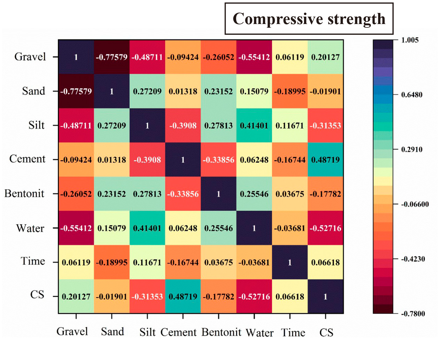
Figure 1. Coefficients of Pearson Correlation for CS.

 

Before modeling, the data were randomly split into testing (30%) and training (70%) parts. Table 1 displays the statistical characteristics of the output and input variables for the testing and training data for CS-BPC. A logical and technical range can be developed for each of the input variables by considering the minimum and maximum for each of the four data sets. In particular, these ranges are 0 to 1,060kg/m3 for gravel; 509 to 1,499kg/m3 for sand; 0 to 380kg/m3 for silty clay; 65 to 300kg/m3 for cement; 16 to 320kg/m3 for bentonite; 152 to 520kg/m3 for water; and 7 to 540 days for curing time. Tables 1 allows you to identify extreme data points (maximum and minimum), data centers (mean and median), data spread (standard deviation and variance), and distribution shapes (skewness and kurtosis)[47]. Moreover, the diversity among databases and the ability of models developed on them to generalize are illustrated by the diverse alterations observed in each of the outputs[12].

 

Table 1. Comprehensive Statistics for Both Testing and Training Data Related to CS-BPC

 

3.2 Model efficiency Assessment Specifications

Several error metrics were employed to assess the accuracy of the models. Among these variables are R2, MAE, RMSE, MAPE, a20-index, and OBJ[13]. These statistical metrics are summarized as follows:

 

$${{R}}^{2}={\left[\frac{{\sum }_{{i}=1}^{{N}}({{Y}}_{{o}{b}{s}}-{\overline{{Y}}}_{{o}{b}{s}})({{Y}}_{{p}{r}{e}}-{\overline{{Y}}}_{{p}{r}{e}})}{\sqrt{{\sum }_{{i}=1}^{{N}}({{Y}}_{{o}{b}{s}}-{\overline{{Y}}}_{{o}{b}{s}}{)}^{2}{\sum }_{{i}=1}^{{N}}({{Y}}_{{p}{r}{e}}-{\overline{{Y}}}_{{p}{r}{e}}{)}^{2}}}\right]}^{2} \left(1\right)$$

$${M}{A}{E}=\frac{{\sum }_{{i}=1}^{{N}}\left|{{Y}}_{{p}{r}{e}}-{{Y}}_{{o}{b}{s}}\right|}{{N}} \left(2\right)$$

$${M}{A}{P}{E}=\frac{{\sum }_{{i}=1}^{{N}}\left|{{Y}}_{{p}{r}{e}}-{{Y}}_{{o}{b}{s}}\right|}{{\sum }_{{i}=1}^{{N}}{{Y}}_{{o}{b}{s}}}\times 100 \left(3\right)$$

$${R}{M}{S}{E}=\sqrt{\frac{1}{{N}}{\sum }_{{i}=1}^{{N}}({{Y}}_{{p}{r}{e}}-{{Y}}_{{o}{b}{s}}{)}^{2}} \left(4\right)$$

$${a}20-{i}{n}{d}{e}{x}=\frac{{m}20}{{N}} \left(5\right)$$

 

when N is the number of records, Ypre and Yobs show the predicted and actual values, and the bar items over the parameters indicate the average rate; The variable m20 shows the records quantity where the Yobs/Ypre ratio ranges from 0.80 to 1.20;

 

3.3 Algorithms for Hybrid Ensemble Learners

The FBIO was used in this study to determine the ideal values using the given criteria to set the first random values (Table 2). After these statistics were entered into EL approaches and the EL algorithms were trained using the training dataset, the objective function was determined to be the average RMSE of both data (test and train). Figure 2 provides a summary of the various EL-FBIO approaches. Table 3 presents the multiple meta-parameters values optimized for CS-PC models.

 

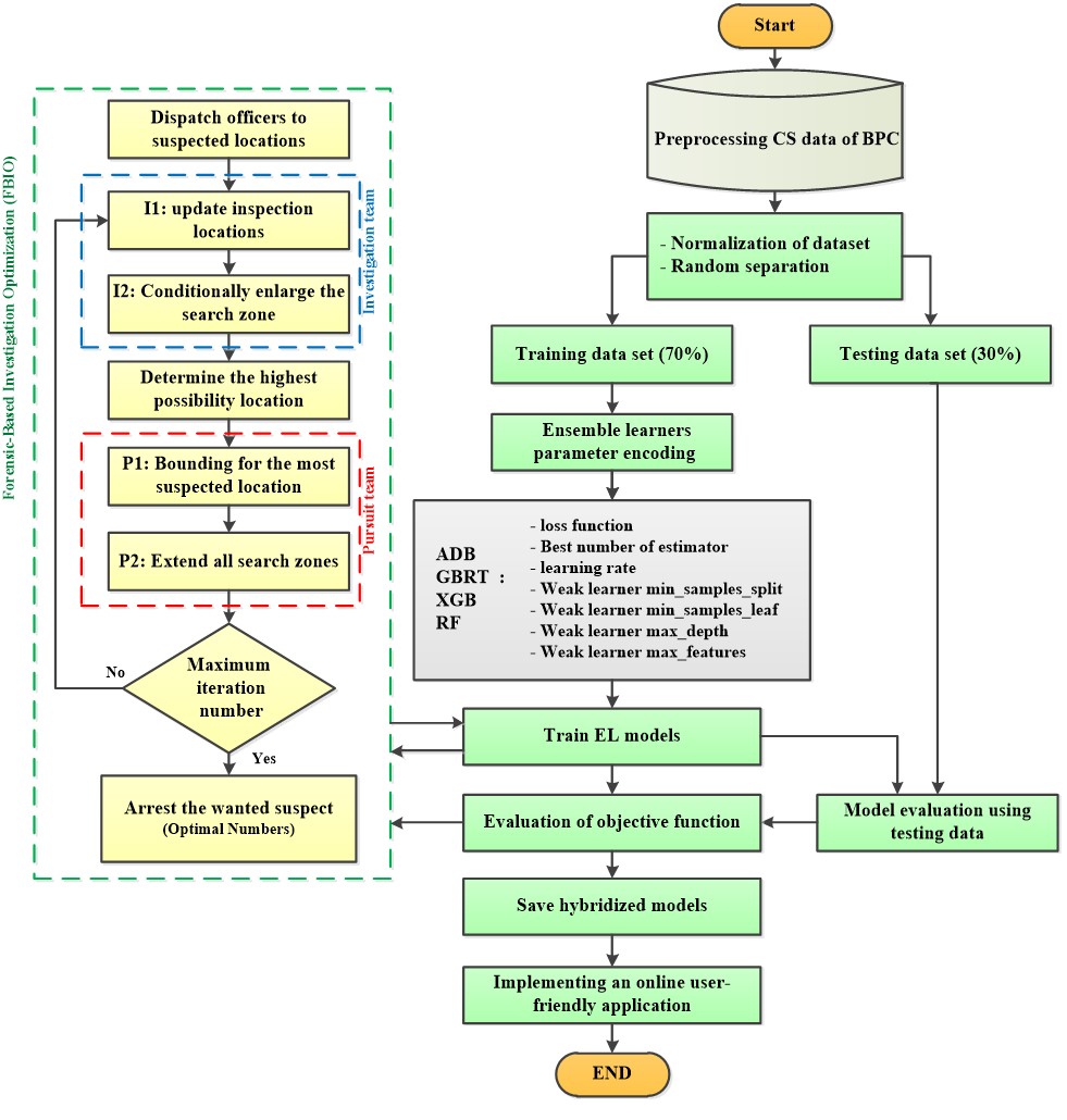
Figure 2. An Overview of The Modeling Process in This Study.

 

Table 2. Different Meta-Parameter Ranges Used in The Optimization Process.

 

Table 3. Optimized Parameter Values for CS-BPC

 

3.4 Model Prediction Accuracy Study

Because of a higher R2-value and fewer scattered spots, the GBRT-FBIO approach outperforms conventional CS-BPC models in both phases of test and train, as shown in Figure 3. A20-index is a new significant engineering parameter that determines how many specimens have expected values that are at most 20% off from observed values[48]. Furthermore, with an a20-index of 0.5 and 0.88 throughout the testing and training step, the RF- FBIO had the lowest desire to perform well for CS-BPC.

 

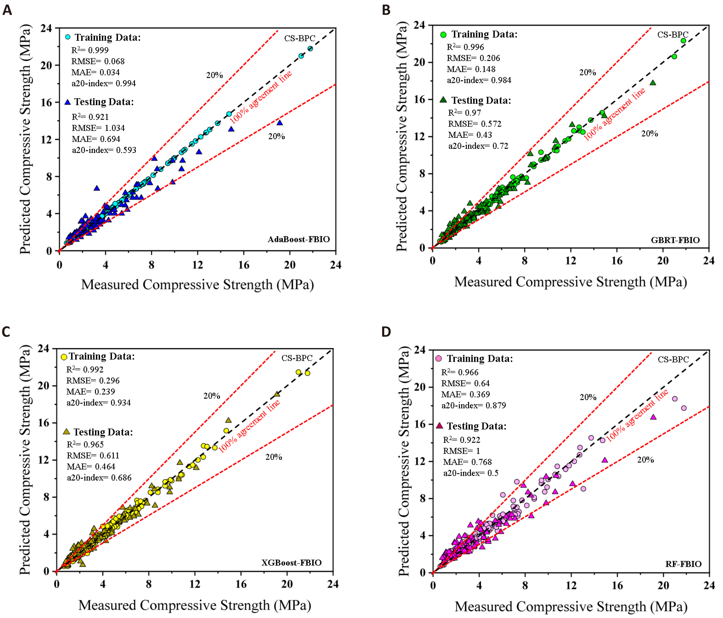
Figure 3. Measured Versus Expected Scattering Dots in the CS-BPC Phases.

 

Different statistical indicators were evaluated for training and testing datasets in order to assess the precision of the proposed forecasting models. Table 4 shows what the results are for different statistical parameters. In the CS-BPC training phase, ADB is 0.14, 0.23, and 0.57MPa lower than GBRT, XGB and RF in terms of RMSE, while in the testing phase, GBRT outperformed ADB, XGB, and RF by 0.46, 0.04, and 0.43MPa of difference in RMSE, respectively. Despite the relative superiority of the ADB model during training, the GBRT model with MAE and MPAE of 0.43 and 0.16 respectively, is the most accurate in testing phase.

 

Table 4. The Precision and Effectiveness of Each CS-FBIO Model

 

The effectiveness of each design was evaluated using the diagram of Taylor presented in Figure 4. To compare the anticipated outcomes with the actual values, three statistical measures of RMSE, STD, and R2) were used. The standard deviation is shown through a circle connecting the plot's axes of horizontal and vertical; RMSE is indicated by the horizontal green dots and the blue line shows the values of R2. As a result, among all techniques for CS-BPC, the GBRT-FBIO and XGB methods have the top performance.

 

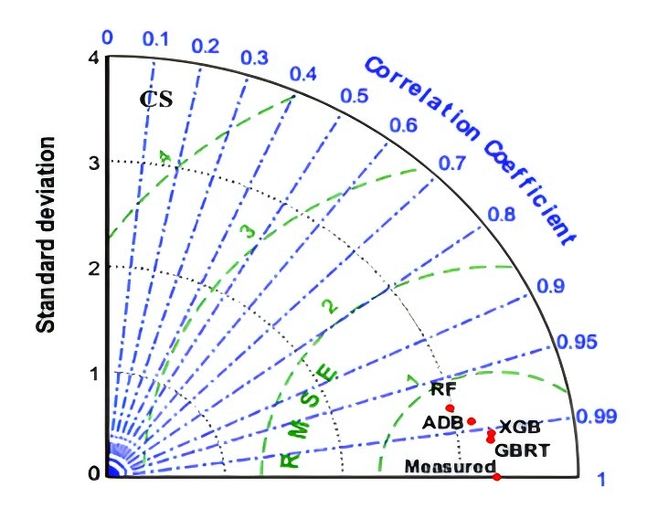
Figure 4. Taylor Graphs of Several CS-FBIO Models and Traditional Approaches.

 

ML and EL models can accurately predict BPC strength and workability properties, as reported by several studies[14,18-21]. According to R2 compare, GBRT methods for CS outperformed all existing models during the testing and training levels. Based on RMSE and MAE values for CS, some existing models were superior, potentially due to the dataset’s quality. As a result, EL methods are more practical and generalize more effectively to BPC characteristics, thus saving time and resources.

 

Table 5. Comparing Proposed El Models to Those in the Literature

 

3.5 SHAP

SHAP is a game-theoretic approach designed to describe the result of machine-learning methods[49]. SHAP presents the contribution of the feature to the mode’s output, offering a more interpretable and transparent understanding of the model’s decision-making process. In the ensuing sections, we thoroughly analyze the outcomes in the proposed predicting structure, which is designed to interpret and comprehend the results of the probabilistic predicting model. Our initial focus is on point forecasts, specifically examining how the developed model utilizes various features to make predictions. The SHAP method is employed for explanations, covering CS. Figure 5 illustrates the average contribution of each feature, with each bar plot representing the importance of a specific property. Cement and water play significant roles in CS model, contributing more substantially. Also, Silt exhibits minimal impact on the outputs.

 

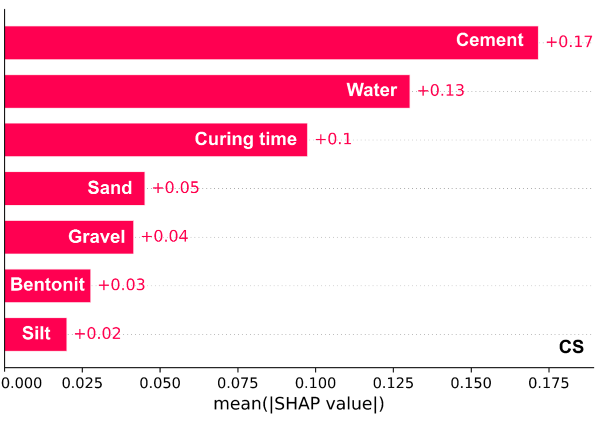
Figure 5. Feature Significance of the Input Variables.

 

Each dot in Figure 6 represents a distinct forecasting, and its location along the x-axis signifies the impact of that attribute on the output of the model. Furthermore, each dot's color corresponds to a feature value (varies from blue to red) emphasizing the relative contributions of different feature values to the final result. The long tails show characteristics that are highly significant. The dots’ vertical distribution suggests that there are more findings with comparable effects. These SHAP summary graphs in such a setting include details on the number of reports that have those qualities as well as the size and direction of each feature's effect. As an example, elevated cement values in CS model tend to elevate the model output, while values closer to zero for cement lead to a decrease in the model output. Therefore, the impact on the model output becomes more substantial with higher cement values.

 

Figure 6. Summary Plot of the Point Predicting Model.

 

A heatmap of SHAP values across all input variables is shown in Figure 7. CS was shown on top as functions of all variables. The ranges of SHAP values which show the impact on each model target are depicted by various colors ranging from blue to red. For this heatmap, arbitrary sample pools equal to training data sets were chosen. Considering the intense 11 on the left side of the CS-BPC, water and cement appear to be two key input parameters.

 

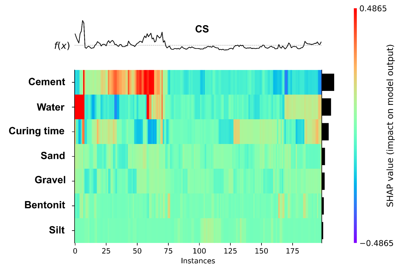
Figure 7. SHAP Values and Function Variations of Each Target.

 

3.6 Online Application of Proposed BPC Models

Models developed using EL-FBIO methods differ from classical regression methods as they do not simply establish direct relationships between inputs and outputs[50]. To address this, implementing an online application would allow researchers and practicing engineers, who are the end users of the proposed BPC models, to easily estimate mechanical and workability properties. Several previous studies have developed software using MATLAB Graphical User Interface to predict the properties of different types of concrete[51,52]. The proposed online application offers several key advantages: (i) faster access to results, enabling more thorough investigation of mix designs; (ii) reduced production costs, while ensuring the safety and quality of concrete designs, by allowing users to determine whether a mix design is reasonable; and (iii) ease of use, which minimizes human error in calculations[37]. Free online access is provided as well (https://colab.research.google.com/drive/1a3pjScLsripH-756yYk2nyol5g7HM9U1), allowing engineers and researchers to obtain accurate predictions of BPC strength and workability parameters directly at their project site in just a few simple steps.

 

3.7 Limitations

The dataset of 285 compressive strength records used in this study is relatively small, which could limit the robustness and generalizability of the machine learning models developed. Small datasets increase the risk of overfitting, where models perform well on the training data but struggle to generalize to new, unseen data. Additionally, the dataset, compiled from various published sources, may contain inherent biases due to variations in material preparation, testing environments, and input parameters. These inconsistencies could affect the model’s ability to accurately predict compressive strength in broader applications. While ensemble models like RF, GBRT, and XGB are generally robust, they are sensitive to the quality and diversity of the input data, and with a limited dataset, they may not capture the full range of variability needed for real-world applications. Cross-validation and regularization techniques were applied to mitigate some of these concerns, but the findings should still be interpreted cautiously. Future work should focus on expanding the dataset through additional experiments or synthetic data generation, and employing uncertainty quantification methods to enhance the reliability and generalizability of the predictions in practical engineering contexts.

 

4 CONCLUSION

This research introduces an advanced machine learning approach for predicting the CS of BPC using Python-based ensemble techniques, including RF, ADB, GBRT, and XGB, all optimized through FBIO algorithms. The challenge of accurately assessing BPC’s compressive strength through experimental or field evaluation lies in the complexity, high costs, and need for professional expertise. To overcome these barriers, this study proposes an improved and accessible computational method, allowing for more efficient and reliable predictions of BPC properties. To build the predictive models, 285 data records of CS tests were collected from a variety of published literature sources. The selected input variables-gravel, bentonite, silty clay, curing time, sand, cement, and water-were used to train the models and assess their performance. A comprehensive evaluation of each model was performed using key performance metrics, including the R², MAE, RMSE, MAPE, and the a20-index, for both the training and test datasets. Among the models, GBRT emerged as the most accurate for predicting BPC compressive strength, consistently outperforming other ensemble methods based on the evaluation metrics. In addition to superior predictive accuracy, the study utilized SHAP to interpret the model’s predictions and provide insights into the relative importance of each input variable. The SHAP analysis demonstrated that cement was the most significant factor influencing BPC’s compressive strength, with a mean SHAP value of 0.17, indicating its substantial impact on model predictions. This insight emphasizes the importance of cement variations in the overall performance of BPC and highlights the practical value of the model in optimizing BPC mix designs. Overall, the findings of this research underscore the potential of ensemble learning methods, particularly GBRT with FBIO optimization, in offering a robust and efficient alternative to traditional testing methods for BPC. The developed models not only reduce the need for expensive and time-consuming experimental evaluations but also provide a practical tool for researchers and engineers to predict BPC properties with high accuracy.

 

As a suggestion for future work, we recommend exploring the application of advanced machine learning techniques, such as deep neural networks (DNNs) and transfer learning, which may enhance model performance, particularly for small datasets. To address scalability concerns, future studies should also investigate the feasibility of applying FBIO to larger datasets or real-time applications by integrating more efficient optimization algorithms, such as Bayesian optimization or genetic algorithms, which could improve hyperparameter tuning while reducing computational costs. Expanding the dataset through additional experiments or synthetic data generation could further improve model generalizability. Additionally, exploring parallel processing or cloud-based computing could help optimize FBIO’s scalability for real-time use. Finally, incorporating uncertainty quantification methods would offer valuable insights into the reliability and robustness of predictions in practical engineering applications.

 

Acknowledgements

Thanks to Dr. Ali Reza Ghanizadeh and Dr. Samer Dessouky, for their invaluable guidance and support.

 

Conflicts of Interest

The authors declared no conflict of interest.

 

Author Contribution

Amlashi AT was responsible for conceptualization, conducting the investigation, providing resources, drafting the original manuscript, and project administration. Ghanizadeh AR contributed to the methodology, validation, software development, visualization, and provided supervision. Dessouky S oversaw the supervision and contributed to the review and editing of the manuscript.

 

Abbreviation List

ADB, Adaptive boosting

AI, Artificial intelligence

ANN, Artificial neural network

BPC, Bentonite plastic concrete

CS, Compressive strength

DT, Decision trees

EL, Ensemble learning

FBIO, Forensic-based investigation optimization

GBRT, Gradient boosting regression tree

ML, Machine learning

OOB, Out-of-bag

RF, Random forest

RSM, Response surface methodology

SHAP, SHapley additive exPlanations

SVM, Support vector machine

XGB, Extreme gradient boosting

 

References

[1] Keramati M, Goodarzi S, Moradi Moghadam H et al. Evaluating the stress–strain behavior of MSW with landfill aging. Int J Environ Sci Technol, 2019; 16: 6885-6894.[DOI]

[2] Pandey G, Madhuri S. Heavy metals causing toxicity in animals and fishes. Res J Anim Vet Fish Sci, 2014; 2: 17-23.

[3] Tytła M. Assessment of heavy metal pollution and potential ecological risk in sewage sludge from municipal wastewater treatment plant located in the most industrialized region in Poland-case study. Int J Environ Res Public Health, 2019; 16: 2430.[DOI]

[4] Liu Q, Zhou Y, Lu J et al. Novel cyclodextrin-based adsorbents for removing pollutants from wastewater: A critical review. Chemosphere, 2020; 241: 125043.[DOI]

[5] Barakan S, Aghazadeh V. The advantages of clay mineral modification methods for enhancing adsorption efficiency in wastewater treatment: a review. Environ Sci Pollut Res, 2021; 28: 2572-2599.[DOI]

[6] Uddin MK. A review on the adsorption of heavy metals by clay minerals, with special focus on the past decade. Chem Eng J, 2017; 308: 438-462.[DOI]

[7] Hussain ST, Ali SAK. Removal of heavy metal by ion exchange using bentonite clay. J Ecol Eng, 2021; 22: 104-111.[DOI]

[8] Thakur AK, Kumar R, Chaudhari P et al. Removal of Heavy Metals Using Bentonite Clay and Inorganic Coagulants. In: Shah MP (eds). Removal of Emerging Contaminants Through Microbial Processes. Springer, Singapore. 2021: 47-69.[DOI]

[9] Abbaslou H. Effects of mix design and curing time on compressive and tensile strength of bentonite plastic concrete. Concrete Res, 2017; 10: 109-124.[DOI]

[10] Bahrami M, Hosseini SMMM. A new incorporative element to modify plastic concrete mechanical characteristics for cut-off wall construction in very soft soil media: Identification of tensile galvanized open-mesh distributer (TGOD) element. Constr Build Mater, 2022; 350: 128884.[DOI]

[11] Athani SS, Solanki C, Dodagoudar G. Seepage and stability analyses of earth dam using finite element method. Aquat Proced, 2015; 4: 876-883.[DOI]

[12] Tavana Amlashi A, Mohammadi Golafshani E, Ebrahimi SA et al. Estimation of the compressive strength of green concretes containing rice husk ash: a comparison of different machine learning approaches. Eur J Environ Civil Eng, 2023; 27: 961-983.[DOI]

[13] Alidoust P, Goodarzi S, Tavana Amlashi A et al. Comparative analysis of soft computing techniques in predicting the compressive and tensile strength of seashell containing concrete. Eur J Environ Civil Eng, 2023; 27: 1853-1875.[DOI]

[14] Ghanizadeh AR, Abbaslou H, Amlashi AT et al. Modeling of bentonite/sepiolite plastic concrete compressive strength using artificial neural network and support vector machine. Front Struct Civ Eng, 2019; 13: 215-239.[DOI]

[15] Li Z, Yim SH-L, Ho K-F. High temporal resolution prediction of street-level PM2. 5 and NOx concentrations using machine learning approach. J Clean Prod, 2020; 268: 121975.[DOI]

[16] Ehteram M, Panahi F, Ahmed AN et al. Inclusive Multiple Model Using Hybrid Artificial Neural Networks for Predicting Evaporation. Front Environ Sci, 2022; 9: 789995.[DOI]

[17] Khan MA, Memon SA, Farooq F et al. Compressive Strength of Fly‐Ash‐Based Geopolymer Concrete by Gene Expression Programming and Random Forest. Adv Civil Eng, 2021; 2021: 6618407.[DOI]

[18] Amlashi AT, Abdollahi SM, Goodarzi S et al. Soft computing based formulations for slump, compressive strength, and elastic modulus of bentonite plastic concrete. J Clean Prod, 2019; 230: 1197-1216.[DOI]

[19] Tavana Amlashi A, Ghanizadeh AR, Abbaslou H et al. Developing three hybrid machine learning algorithms for predicting the mechanical properties of plastic concrete samples with different geometries. AUT J Civil Eng, 2020; 4: 37-54.[DOI]

[20] Amlashi AT, Alidoust P, Ghanizadeh AR et al. Application of computational intelligence and statistical approaches for auto-estimating the compressive strength of plastic concrete. Eur J Environ Civ En, 2022; 26: 3459-3490.[DOI]

[21] Alishvandi A, Karimi J, Damari S et al. Estimating the compressive strength of plastic concrete samples using machine learning algorithms. Asian J Civil Eng, 2024; 25: 1503-1516.[DOI]

[22] Li Q-F, Song Z-M. High-performance concrete strength prediction based on ensemble learning. Constr Build Mater, 2022; 324: 126694.[DOI]

[23] Feurer M, Hutter F. Hyperparameter optimization. In: Hutter F, Kotthoff L, Vanschoren J (eds). Automated Machine Learning. The Springer Series on Challenges in Machine Learning. Springer, Cham. 2019: 3-33.[DOI]

[24] Duan J, Asteris PG, Nguyen H et al. A novel artificial intelligence technique to predict compressive strength of recycled aggregate concrete using ICA-XGBoost model. Eng Comput, 2021; 37: 3329-3346.[DOI]

[25] Yang L, Shami A. On hyperparameter optimization of machine learning algorithms: Theory and practice. Neurocomputing, 2020; 415: 295-316.[DOI]

[26] Qu Z, Liu H, Wang Z et al. A combined genetic optimization with AdaBoost ensemble model for anomaly detection in buildings electricity consumption. Energy Build, 2021; 248: 111193.[DOI]

[27] Moghaddam HM, Keramati M, Fahimifar A et al. Shear modulus prediction of landfill components using novel machine learners hybridized with forensic-based investigation optimization. Constr Build Mater, 2024; 411: 134443.[DOI]

[28] Schapire RE. The strength of weak learnability. Mach Learn, 1990; 5: 197-227.[DOI]

[29] Freund Y, Schapire R, Abe N. A short introduction to boosting. J Jpn Soc Artif Intelli, 1999; 14: 1612.

[30] Nisar N, Bhat JA. Experimental investigation of Rice Husk Ash on compressive strength, carbonation and corrosion resistance of reinforced concrete. Aust J Civil Eng, 2021; 19: 155-163.[DOI]

[31] Shang M, Li H, Ahmad A et al. Predicting the mechanical properties of RCA-based concrete using supervised machine learning algorithms. Materials, 2022; 15: 647.[DOI]

[32] Breiman L, Friedman J, Olshen RA et al. Classification and Regression Trees. Routledge, 2017.[DOI]

[33] He Q, Kamarianakis Y, Jintanakul K et al.  Incident Duration Prediction with Hybrid Tree-based Quantile Regression. In: Ukkusuri S, Ozbay K (eds). Advances in Dynamic Network Modeling in Complex Transportation Systems. Complex Networks and Dynamic Systems, Springer, New York, USA. 2013: 287-305.[DOI]

[34] Chen T, He T, Benestyc M et al. Xgboost: extreme gradient boosting. R package version 0.4-2, 2015; 1: 1-4.

[35] Svetnik V, Liaw A, Tong C et al. Random Forest:  A Classification and Regression Tool for Compound Classification and QSAR Modeling. J Chem Inf Comput Sci, 2003; 43: 1947-1958.[DOI]

[36] Farooq F, Nasir Amin M, Khan K et al. A comparative study of random forest and genetic engineering programming for the prediction of compressive strength of high strength concrete (HSC). Appl Sci, 2020; 10: 7330.[DOI]

[37] Chou J-S, Chen L-Y, Liu C-Y. Forensic-based investigation-optimized extreme gradient boosting system for predicting compressive strength of ready-mixed concrete. J Comput Des Eng, 2023; 10: 425-445.[DOI]

[38] Abbaslou H, Ghanizadeh AR, Amlashi AT. The compatibility of bentonite/sepiolite plastic concrete cut-off wall material. Constr Build Mater, 2016; 124: 1165-1173.[DOI]

[39] Hu LM, Gao DY, Li YZ et al. Analysis of the influence of long curing age on the compressive strength of plastic concrete. Adv Mater Res, 2012; 382: 200-203.[DOI]

[40] Pashang Pisheh Y, Mir Mohammad Hosseini S. Stress-strain behavior of plastic concrete using monotonic triaxial compression tests. J Cent South Univ, 2012; 19: 1125-1131.[DOI]

[41] Tahershamsi A, Bakhtiary A, Binazadeh N. Effects of clay mineral type and content on compressive strength of plastic concrete. J Min Eng, 2009; 4: 35-42.

[42] Guan QY, Zhang P. Effect of clay dosage on mechanical properties of plastic concrete. Adv Mater Res, 2011; 250: 664-667.[DOI]

[43] Zhang P, Guan Q, Li Q. Mechanical properties of plastic concrete containing bentonite. Res J Appl Sci Eng Technol, 2013; 5: 1317-1322.[DOI]

[44] Mahboubi A, Ajorloo A. Experimental study of the mechanical behavior of plastic concrete in triaxial compression. Cement Concrete Res, 2005; 35: 412-419.[DOI]

[45] Pashazadeh A, Chekani-Azar M. Estimating an appropriate plastic concrete mixing design for cutoff walls to control leakage under the earth dam. J Basic Appl Sci Res, 2011; 1: 1295-1299.

[46] Elwell DJ, Fu G. Compression testing of Concrete: Cylinders vs. Cubes. Transportation Research and Development Bureau, New York, USA. 1995.

[47] Iqbal MF, Liu Q-f, Azim I et al. Prediction of mechanical properties of green concrete incorporating waste foundry sand based on gene expression programming. J Hazard Mater, 2020; 384: 121322.[DOI]

[48] Asteris PG, Ashrafian A, Rezaie-Balf M. Prediction of the compressive strength of self-compacting concrete using surrogate models. Comput Concr, 2019; 24: 137-150.[DOI]

[49] Lundberg S, Lee SI. A Unified Approach to Interpreting Model Predictions. arXiv:1705.07874, 2017.[DOI]

[50] Heidarabadizadeh N, Ghanizadeh AR, Behnood A. Prediction of the resilient modulus of non-cohesive subgrade soils and unbound subbase materials using a hybrid support vector machine method and colliding bodies optimization algorithm. Constr Build Mater, 2021; 275: 122140.[DOI]

[51] Golafshani EM, Behnood A. Estimating the optimal mix design of silica fume concrete using biogeography-based programming. Cement Concrete Comp, 2019; 96: 95-105.[DOI]

[52] Golafshani EM, Behnood A. Application of soft computing methods for predicting the elastic modulus of recycled aggregate concrete. J Clean Prod, 2018; 176: 1163-1176.[DOI]

 

Copyright © 2024 The Author(s). This open-access article is licensed under a Creative Commons Attribution 4.0 International License (https://creativecommons.org/licenses/by/4.0), which permits unrestricted use, sharing, adaptation, distribution, and reproduction in any medium, provided the original work is properly cited.