Mathematical Models of Wound Healing and Tissue Regeneration: Insights with Numerical Solution

 

Geeta Arora1#, Sarabjit Singh2#, Homan Emadifar3#*

 

1Department of Mathematics, Lovely Professional University, Punjab, India

2Department of General Surgery, Punjab Institute of Medical Sciences, Jalandhar, Punjab, India

3Department of Mathematics, Hamedan Branch, Islamic Azad University, Hamedan, Iran

 

#These authors contributed equally to this work and should be considered co-first authors.

 

*Correspondence to: Homan Emadifar, PhD, Department of Mathematics, Hamedan Branch, Islamic Azad University, Hamedan,009881, Iran; E-mail: homan_emadi@yahoo.com

 

DOI: 10.53964/id.2024013

 

Abstract

Understanding and forecasting the dynamics of wound healing processes heavily relies on mathematical modeling. Researchers can understand the complicated connections between cells, tissues, and biochemical components involved in wound healing by using mathematical equations and computational simulations. One such mathematical model that has seeks the interest of researchers in exploring wound healing phenomenon is Fisher’s equation. In the present work, the equation is solved using differential quadrature method with trigonometric tension B-spline (TTBs) basis function. The obtained results are compared with the results obtained from earlier studies and the results are presented in form of tables and figures. The implementation of the particle swarm optimization algorithm has removes the dilemma of unknown parameter involvement in the TTBs and hence resulted in a novel technique to find the numerical results.

 

Keywords: wound healing, Fisher's equation, differential quadrature method, B spline, particle swarm optimization

 

1 INTRODUCTION

To understand the biological processes the mathematical modeling plays a very important role. Wound healing is a process of recovering of an injured tissue. It is a multifaceted biological phenomenon that arises as a natural response to the damaged tissue. Directed migration, or the movement of cells towards the wound, is one of the key elements in wound healing. There are various aspects of wound healing that can be covered with the involvement of study with mathematical modelling.

 

The first aspect is that the mathematical models provide insight into wound healing mechanisms. These models facilitate the integration of experimental and clinical data, resulting in a thorough comprehension of the underlying cellular and molecular processes. They cast light on important factors including cell migration, proliferation, differentiation, angiogenesis, extracellular matrix remodeling, and inflammation.

 

The second aspect is the predictive ability of mathematical models in wound healing[1]. These models estimate wound closure rates and predict healing times by simulating the progression of wound healing under various conditions. This predictive ability helps clinicians evaluate wound healing trajectories, design treatment strategies, and manage patient expectations.

 

In order to better understand the biological process of mathematical modelling associated with the wound healing, this paper discusses the importance of Fisher’s equation, which is a equation that exists as a mathematical modelling of this phenomenon. To numerically solve the equation, the differential quadrature method (DQM) is applied to the equation using trigonometric tension B-spline (TTBs) functions. It also utilizes one of the well-known optimization technique, particle swarm optimization (PSO) technique to minimize the error in the solution based on the parameter value. The novelty of the work includes the implementation of the DQM with the optimization technique that leads to the error minimization. The present research is actually creating a new way of using the optimization to minimize the error involved in the numerical methods.

 

2 METHODS

2.1 Existing Mathematical Models in Wound Healing Process

There are different types of studies based on mathematical models used in the study of wound healing such as cell-based models illustrate how individual cells behave and interact during wound healing. To mimic cell migration, proliferation, and differentiation, these models frequently employ agent-based modelling or cellular automaton techniques. They can record cell distribution and reactions to biochemical signals in the wound microenvironment[2].

 

There are reaction-diffusion models that describes the diffusion and reactivity of biochemical substances in the wound site, such as growth factors or cytokines. These models include equations that describe molecular transport and interactions with cells and tissues. The continuum models, are the models frequently based on partial differential equations (PDEs), that describe wound healing processes in a continuous manner[3]. These models take into account the distribution and changes in critical variables throughout time and space, such as cell density, extracellular matrix components, and growth factors.

 

One of the models[3] to discuss the density of cells at a particular instant of time is defined as follows:

 

 

where the cell layer is presented as a two-dimensional compressible fluid.

 

Here, ν is considered as a constant appearing from the ratio of the proportionality constant and adhesion constant. the growth term, denoted as g(u) characterizes the density-dependent net rate of change in the quantity of cells within the layer as a result of both proliferation and perish. In the context of modelling enterocyte migration experiments, the term g(u) is commonly regarded as zero. Similarly, when modelling cell-colony expansion, it is assumed that g(u) follows a logistic growth pattern. In this context, the boundary conditions are considered based on the scenario of wound closure.

 

The mechanical models examine the function of mechanical forces in wound healing, such as tension and compression[4]. To describe the mechanical properties of tissues and their reaction to external forces, these models frequently combine notions from continuum mechanics. Ordinary differential equations (ODEs) are often used to describe discrete models. These equations don't have to be solved for the whole domain. Instead, they are solved locally to predict how each object will change over time.

 

In general, there exist some hybrid models also that employ many modelling methodologies to represent multiple elements of wound healing. A hybrid model, for example, may combine a cell-based model with reaction-diffusion model to simulate cell-biochemical component interactions. These models enable a more comprehensive description of the intricate wound healing processes.

 

The field of mathematical modelling in wound healing is dynamic, with advances and modifications being made to better reflect the complexity of the healing process[5]. Figure 1 presents the different types of mathematical models that has been used to discuss the wound healing.

 

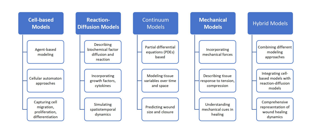
Figure 1. Types of Mathematical Models in the Study of Wound Healing.

 

Mathematical modelling of wound healing has been extensively studied and documented in the literature. A variety of features of wound healing, including as the cellular and molecular processes involved, the interactions between various cell types, the impacts of biochemical variables and treatments, and the overall dynamics of wound closure, have been described and simulated using mathematical models. Figure 2 presents an explanation of the function of mathematical modelling in wound healing.

 

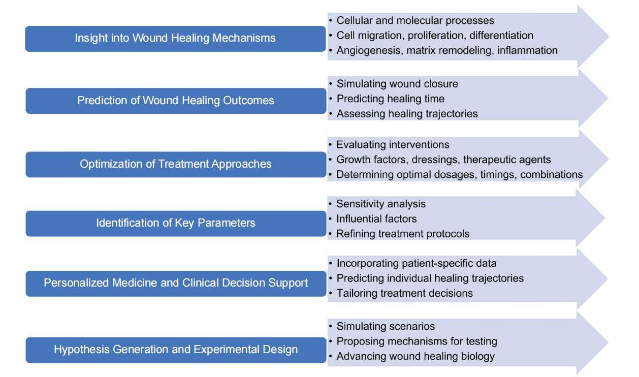
Figure 2. Mathematical Modeling in Wound Healing.

 

In a study by Jorgensen and Sanders[6], a summary of mathematical models is provided that focus to study wound healing processes. Different modelling approaches, including cell-based models, reaction-diffusion models, and continuum models, are discussed. The work highlights the contributions of mathematical modelling to the elucidation of the role of important factors in wound healing, including cell migration, proliferation, and angiogenesis.

 

Modelling biological processes, such as inflammation and wound healing, uses differential equations more frequently than any other standard, classical technique. All stages of wound healing, from inflammation to wound closure, have been studied using equation-based models. These computational models have been studied to serve as the foundation for personalized preventive interventions[7].

 

In 2021, a review has been reported to explore the mathematical models of skin wound healing[8]. This article provides an overview of the different ways in which mathematical modelling can provide profound insights into the mechanisms that underlie aspects of wound healing, encompassing seminal works from the last several decades as well as contemporary advancements in the field. The contributions of these models have been highlighted and made to the understanding of the interplay between the multitude of components underlying the healing process, as well as to the development of more effective treatment strategies.

 

2.2 Fisher Equation

Fisher published the Fisher’s equation, a reaction-diffusion equation, in 1937[9] to analyze the expansion of beneficial genes brought about by mutation. Subsequently, extensive research has been conducted to explore the use of this equation in other phenomena, such as the emergence of patterns in the propagation of waves, the examination of cellular growth in the field of tissue engineering, the modelling of oscillatory chemical reactions, population biology, wound healing, and the progression of tumors.

 

The Equation (2) is a nonlinear which is named as Fisher’s reaction diffusion equation with the right hand expanded as follows:

 

 

Here, the variables of the equation correspond to the constituent elements of the phenomenon elucidated by Fisher’s equation. The interpretation of u(x,t), depends on the specific application of the equation. For example, in the context of brain tumour analysis, the variable u(x,t), represent the carrying capacity, v denotes cell mobility as indicated by the diffusion coefficient, and r signifies the growth rate.

 

While in the framework of wound healing, the variable u, denoted as u(x,t), reflects the number of cells at a specific spatial location x and time t. The initial component on the right-hand side of the equation reflects spatial diffusion with a diffusion rate denoted as ν, whereas the subsequent term signifies the population's logistic growth[9].

 

In recent years, academics have undertaken numerous endeavours to ascertain the precise solution to the equation by both analytical and numerical methods. For example, the equation was subjected to numerical analysis[10] via the moving mesh approach. A comparative analysis[11] was conducted to evaluate the non-standard finite-difference scheme (FDS) and nodal integral approach using the finite element numerical solution. The Adomian decomposition approach[12] was utilized to show the precise numerical solution of the problem analytically. In a study, a puesudospectral strategy is proposed[13] that utilizes Chebyshev-Lobatto points for the purpose of solving the problem. The Fisher’s equation is solved using a DQM[14] with FDS implementation. Additional numerical techniques, such as the radial basis function based Pseudospectral method[15] and the DQM[16], have been effectively employed in recent years to obtain the numerical solution of Fisher’s equation. Various other computational techniques have also been employed by researchers to ascertain the numerical solution to Fisher reaction diffusion equations. These techniques include a sinc collocation method[17], a B-spline collocation method[18], a modified cubic B-spline collocation method[19], a Crank-Nicolson based hybrid approach with DQM[20], and B-spline with finite element approach[21].

 

2.3 Methodology

The DQM, first proposed by Bellman et al.[22] in their seminal work, is a highly effective approach for solving PDEs. In recent times, the DQM has gained significant popularity as a means of determining the weighting coefficients through the utilization of diverse basis functions.

 

The utilizations of B-spline basis functions in various formulations have proven to be effective in addressing PDEs[23-26]. The TTBs is a basis function that has received limited attention in the literature. The implementation of the TTBs functions is done last few years to solve some well-known equations such as the basis functions are used to solve the fractional Burgers’ equation using TTBs with the collocation approach[27], to obtain the extremum of the functionals in calculus of variations[28], to solve the Burger-Huxley equation using the hyperbolic-trigonometric tension B-spline method[29]. Recently, a comparison is made for the trigonometric and hyperbolic tension B-spline[30] to solve hyperbolic telegraph equation.

 

The limited usage of this B-spline can be attributed to the unknown parameter involved that play a major role in finding the numerical solution. To deal with the unknown parameter authors have used the optimization as a tool to obtain the parameter that has proven to be an effective way to obtain the solution of PDE[31,32]. The present study used the widely recognized PSO optimization technique to determine the tension parameter that could results in the minimum error.

 

The DQM involves the transformation of PDE to ODE. The PDE to be solved is transformed to an ODE by expressing the derivatives existing in the equation as the linear sum of the chosen basis function with weighting coefficients the solution is obtained. For instance, the PDE ut = vuxx + ru(1-u),can be written as ut = f(u) once the derivatives of u w..r.t x are written as a linear sum of functions using a basis function. The methodology in detail is discussed as follows:

 

Let [a, b] represents the considered finite domain of the differential equation. This domain can be discretized into a number of known points with a uniform partition having the knots such that:

 

 

with space step as .

 

In DQM, the rth derivative of the function can be approximated as

 

 

Where are the weighing coefficients.

 

The values of can then be utilized to determine the weighting coefficients for the second-order derivatives using the following relationship:

 

 

Let TTB(x) be the B-splines[27,29] fitted on the points distributed uniformly on the knots in the interval [a,b] defined as

 

 

Here p is a tension parameter, s=ph and . The values of the spline and its first two derivatives at the knots xi's are calculated as shown in Table 1.

 

Table 1. TTBs Values

 

Here,

 

Following is the matrix system Aqij=B that results to determine the weighting coefficients for different knot points using the relation for the first order derivative as . With i and j varies from 1 to N denoting the N knots.

 

Here Ψk(xi) are the modified TTRs defined on the first two and the last two points separately to avoid the ill conditioning of the obtained matrix system. Following are the modifications done on the TTBs:

 

 

where i varies from 1 to N for all the knot points.

 

Here A is the coefficient matrix that correspond to each knot point to determine qij’s with the right-hand side defined as the corresponding column of the matrix B shown as:

 

 

Once the derivatives are obtained using the weighting coefficients, the system can be solved that leads to a system of ODEs. There exist multiple methodologies for solving this system of ODEs. Here, the solution is obtained optimal four-stage, order three strong stability-preserving time-stepping Runge-Kutta (SSP-RK43) technique[26], which was our preferred method.

 

Once the solution is obtained it is calculated for the different values of the unknown parameter using the PSO to minimize the errors. An optimization technique is necessary to find the parameters that make the solution better as compared to the results obtained by hit and trial method. PSO[33] is one of the most well-known metaheuristic optimization algorithms, having been successfully deployed in a variety of applications ranging from image processing to finding shape parameter[34,35].

 

The aforementioned algorithm is known for its efficacy, and is influenced by natural phenomena such as fish schools and bird flocks, wherein cooperative behaviors result in outcomes that are considered optimal. Every particle in PSO modifies its trajectory according to its own and neighboring events, promoting collaboration and knowledge acquisition. These particles stand in for potential solutions and change their behavior in a population-based search dependent on their current location and environmental factors.

 

The search process in this technique is driven by the updating of particle positions and velocities at each time step, which is a component of the solution that has to be optimized at each location. Every particle navigates based on its most familiar positions, both within its immediate vicinity and throughout the search area. These positions are modified when other particles uncover new positions. The updating rules for each particle's location and speed are determined using the following relation:

 

 

Where , represents particle’s position and represents i th particle’s velocity in D dimension at time step t, pgb represents the particle having the best fitness value, pib is the particle’s best position visited so far, d1, d2 are acceleration coefficients which quantify particle personal and global experience respectively, x is called constriction coefficient which evaluates a value in the range [0,1] and is given by

 

 

with θ=θ1+θ2, θ1=d1r1, θ2=d2r2 and κ ≈ 1.

 

PSO is an approach employed to iteratively improve parameter values in order to minimize error. The reliability of the solution achieved through the application of the approach is demonstrated by its ability to search for the optimal number of iterations, given a predefined population size or swarm size, and a range of optimized parameters. The parameters considered in this study are as follows: the size of the swarm is set to 10, the maximum number of iterations is set to 50, and the inertia weight is linearly lowered with a value of d1=d2=2.05.

 

The programming in MATLAB is performed using DQM with TTBs and thus calling the PSO for the investigation of parameter leading to the minimization of errors.

 

3 RESULTS AND DISCUSSION

The Fisher’s equation has been considered as a wound healing equation in various form in literature for which the researchers are continuously putting efforts to discuss the underlying phenomenon[36,37]. In this work the equation has been solved by implementation of the above discussed methodology for the different cases as per the value of the reaction factor. Since, the evaluation of error norms allows to study the comparison of the accuracy and efficiency of the numerical methods. The results are presented in form of errors with comparison with the exact solution and the results available from the literature.

 

The application of the Fisher equation is suitable when considering diffusion and proliferation as the primary mechanisms involved in the process of wound healing. Equation (1) defines the variable u(x,t) as the representation of cell density at a certain distance x from the wound edge at time t. The parameter r denotes the proliferation rate of a cell in an environment without crowding, while the constant parameter v represents the diffusivity coefficient for individual cells. The analytical solution for the aforementioned differential equation was derived by Ablowitz and Zepetella[38] as follows:

 

 

The solution of the equation has been obtained considering the domain [-0.2, 0.8] with nonlocal boundary conditions as u(-0.2, t)=1, u(0.8, t)=0. The obtained numerical solutions have been presented in form of figures and tables with the comparison of solutions obtained other schemes from literature. The solution is obtained for the small-time t=0.001 to t=0.002 and with a large value of reaction factor considering the diffusion rate ν=1.

 

The maximum absolute error (L∞) in the numerical and exact solutions are presented in Tables 2 and 3. The values are obtained at different number of subintervals and for different values of parameter of the TTBs for as 2,000 and 10,000 respectively. The considered values of the parameter are obtained using PSO with the number of iterations as 50, the parameter range as [1,5]. The results are obtained with the results available in literature to solve this specific problem.

 

Table 2. L∞ Errors for r=2,000 for Time Step 1×10-5

 

Table 3. L∞ Errors for r=10,000 for Time Step 1×10-5

 

In order to facilitate a comparison between the obtained results and the precise solution, the findings are visually represented through graphical means in Figure 3. The results obtained using the present method demonstrate good accuracy and efficiency for the Fisher's equation. However, for problems with intricate geometries or solutions with sharp gradients, advanced discretization techniques like Discontinuous Galerkin Methods or Adaptive Mesh Refinement could be explored in future work. These methods may provide even higher accuracy and potentially improve efficiency when dealing with complex wound healing scenarios.

 

While numerical methods have proven valuable in simulating wound healing, limitations exist. These limitations can stem from the complexity of biological processes not fully captured by the models, such as the intricate interplay between cell types and the influence of the immune system. Additionally, accurately representing the dynamic changes in the wound environment, including variable tissue properties and blood flow, can be computationally challenging. Furthermore, the effectiveness of a chosen numerical method can be impacted by the specific wound geometry and the desired level of resolution. Despite these limitations, ongoing research continues to refine numerical models and explore advanced computational techniques, aiming to bridge the gap between simulations and the remarkable complexities of wound healing.

 

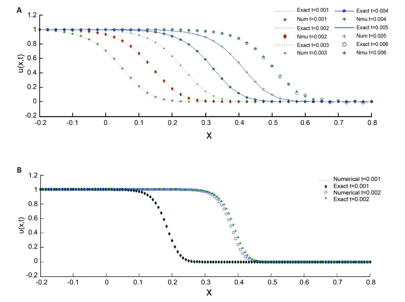
Figure 3. A visual representation illustrating the relationship between time-dependent profiles at various time levels for r=2,000 (A) and r=10,000 (B).

 

4 CONCLUSION

In this study, the PSO technique of optimization has been used to obtain the parameter for the trigonometric tension B-spline-based DQM. This method is employed for the computation of the numerical solution to Fisher’s equation, which finds practical application in the field of wound healing. In order to validate the efficacy of the technique, the problems are addressed using on different values of reaction factors. In order to demonstrate the errors, various time steps and domain partitions are considered. By application of the present method, researchers and scientists can understand the complex interactions that occur during wound healing involving tissues, cells, and biological elements. This study highlights the need of employing interdisciplinary methodologies to enhance our comprehension of intricate biological phenomena and presents opportunities for additional investigation and advancement in the realm of wound healing.

 

Acknowledgements

Not applicable.

 

Conflicts of Interest

The authors declared no conflict of interest.

 

Data Availability

The data generated in this study is in the form of the errors while solving the numerical problems that has been presented in the work in form of tables using the programming in MATLAB.

 

Author Contribution

The work submitted for the publication is a joint effort of the authors. Arora G has formulated the concept of problem solving of the mathematical model with the insight by Sarabjit S related to the wound healing process in support with Emadifar H.

 

Abbreviation List

DQM, Differential quadrature method

FDS, Finite-difference scheme

ODEs, Ordinary differential equations

PDEs, Partial differential equations

PSO, Particle swarm optimization

TTBs, Trigonometric tension B-spline

 

References

[1] Kreger J. On mathematical modeling of epidermal wound healing. Accessed February 2024. Available at:[Web]

[2] Nardini JT, Bortz DM. Investigation of a Structured Fisher's Equation with Applications in Biochemistry. Siam J Appl Math, 2018; 78: 1712-1736.[DOI]

[3] Arciero JC, Mi Q, Branca MF et al. Continuum model of collective cell migration in wound healing and colony expansion. Biophys J, 2011; 100: 535-543.[DOI]

[4] Buganza Tepole A, Kuhl E. Systems-based approaches toward wound healing. Pediatr Res, 2013; 73, 553-563.[DOI]

[5] Maini PK, McElwain DLS, Leavesley D. Travelling waves in a wound healing assay. Appl Math Lett, 2004; 17: 575-580.[DOI]

[6] Jorgensen SN, Sanders JR. Mathematical models of wound healing and closure: a comprehensive review. Med Biol Eng Comput, 2016; 54, 1297-1316.[DOI]

[7] Ziraldo C, Mi Q, An G et al. Computational modeling of inflammation and wound healing. Adv Wound Care, 2013; 2: 527-537.[DOI]

[8] Menon SN, Flegg JA. Mathematical modeling can advance wound healing research. Adv Wound Care, 2021; 10: 328-344.[DOI]

[9] Fisher RA. The wave of advance of advantageous genes. Ann Hum Genet, 1937; 7: 355-369.[DOI]

[10] Qiu Y, Sloan DM. Numerical solution of Fisher's equation using a moving mesh method. J Comput Phys, 1998; 146, 726-746.[DOI]

[11] Rizwan U. Comparison of the nodal integral method and non-standard finite-difference scheme for the Fisher’s equation. Siam J Sci Comput, 2001; 22: 1926-1942.[DOI]

[12] Wazwaz AM, Gorguis A. An analytic study of Fisher's equation by using Adomian decomposition method. Appl Math Comput, 2004; 154: 609-620.[DOI]

[13] Olmos D, Shizgal BD. A pseudospectral method of solution of Fisher's equation. J Comput Appl Math, 2006; 193: 219-242.[DOI]

[14] S AV, Awasthi A. Polynomial based differential quadrature methods for the numerical solution of fisher and extended Fisher–Kolmogorov equations. Int J of Appl Comput Math, 2017; 3: 665-677.[DOI]

[15] Arora G, Bhatia GS. A meshfree numerical technique based on radial basis function pseudospectral method for Fisher’s equation. Int J Nonlin Sci Num, 2020; 21: 37-49.[DOI]

[16] Arora G, Joshi V. A computational approach for solution of one dimensional parabolic partial differential equation with application in biological processes. Ain Shams Eng J, 2018; 9: 1141-1150.[DOI]

[17] Al-Khaled K. Numerical study of Fisher's reaction–diffusion equation by the Sinc collocation method. J Comput Appl Math, 2001; 137: 245-255.[DOI]

[18] Mittal RC, Arora G. Efficient numerical solution of Fisher's equation by using B-spline method. Int J Comput Math, 2010; 87: 3039-3051.[DOI]

[19] Mittal RC, Jain RK. Numerical solutions of nonlinear Fisher's reaction–diffusion equation with modified cubic B-spline collocation method. Math Sci, 2013; 7: 12.[DOI]

[20] Arora G, Mishra S, Singh BK. Nonlinear dynamics of the Fisher's equation with numerical experiments. Nonlinear Stud, 2022; 29: 665-675.

[21] Kırlı E, Irk D. Efficient techniques for numerical solutions of Fisher’s equation using B-spline finite element methods. Comp Appl Math, 2023; 42: 151.[DOI]

[22] Bellman R, Kashef BG, Casti J. Differential quadrature: a technique for the rapid solution of nonlinear partial differential equations. J Comput Phys, 1972; 10: 40-52.[DOI]

[23] Kapoor M, Joshi V. Solution of non-linear Fisher’s reaction-diffusion equation by using Hyperbolic B-spline based differential quadrature method. J Phy, 2019; 1531: 012064.[DOI]

[24] Shukla HS, Tamsir M. Extended modified cubic B-spline algorithm for nonlinear Fisher’s reaction-diffusion equation. Alex Eng J, 2016; 55: 2871-2879.[DOI]

[25] Tamsir M, Huntul MJ. A numerical approach for solving Fisher’s reaction–diffusion equation via a new kind of spline functions. Ain Shams Eng J, 2021; 12: 3157-3165.[DOI]

[26] Arora G, Singh BK. Numerical solution of Burgers’ equation with modified cubic B-spline differential quadrature method. Appl Math Comput, 2013; 224: 166-177.[DOI]

[27] Singh BK, Gupta M. Trigonometric tension B-spline collocation approximations for time fractional Burgers’ equation. J Ocean Eng Sci 2022 (in press).

[28] Alinia N, Zarebnia M. Trigonometric tension B-spline method for the solution of problems in calculus of variations. Comput Math and Math Phys, 2018; 58: 631-641.[DOI]

[29] Alinia N, Zarebnia M. A numerical algorithm based on a new kind of tension B-spline function for solving Burgers-Huxley equation. Numer Algorithms, 2019; 82: 1121-1142.[DOI]

[30] Kapoor M. A comparative study for the numerical approximation of 1D and 2D hyperbolic telegraph equations with UAT and UAH tension B-spline DQM. Nonlinear Eng, 2023; 12: 20220280.[DOI]

[31] Arora G, Chauhan P, Asjad, MI et al. Particle Swarm Optimization for Solving Sine-Gordan Equation. Comput Syst Sci Eng, 2023; 46.[DOI]

[32] Arora G, Kaur H, Emadifar H et al. Forecasting Pollution Using Numerical Simulation Implementing Artificial Bee Colony Optimization. Discrete Dyn Nat Soc, 2023; 2023: 1-10.[DOI]

[33] Wang D, Tan D, Liu L. Particle swarm optimization algorithm: an overview. Soft Comput, 2018; 22: 387-408.[DOI]

[34] Omran M, Engelbrecht AP, Salman A. Particle swarm optimization method for image clustering. Int J Pattern Recogn, 2005; 19: 297-321.[DOI]

[35] Koupaei JA, Firouznia M, Hosseini SMM. Finding a good shape parameter of RBF to solve PDEs based on the particle swarm optimization algorithm. Alex Eng J, 2018; 57: 3641-3652.[DOI]

[36] Fadai NT, Simpson MJ. New travelling wave solutions of the Porous–Fisher model with a moving boundary. J Phys A-Math Theor, 2020; 53: 095601.

[37] İnan B. The Generalized Fractional-Order Fisher Equation: Stability and Numerical Simulation. Symmetry, 2024; 16: 393.[DOI]

[38] Ablowitz MJ, Zeppetella A. Explicit solutions of Fisher's equation for a special wave speed. B Math Biol, 1979; 41: 835-840.[DOI]

 

Copyright © 2024 The Author(s). This open-access article is licensed under a Creative Commons Attribution 4.0 International License (https://creativecommons.org/licenses/by/4.0), which permits unrestricted use, sharing, adaptation, distribution, and reproduction in any medium, provided the original work is properly cited.