
Non-Hermitian Systems with a Real Spectrum and Selective Skin Effect
Li Ge1, 2*
1Department of Physics and Astronomy, College of Staten Island, CUNY, Staten Island, NY, USA
2The Graduate Center, CUNY, New York, NY, USA
*Corresponding to: Li Ge, PhD, Professor, Department of Physics and Astronomy, College of Staten Island, CUNY, 10314, USA; Email: li.ge@csi.cuny.edu
DOI: 10.53964/id.2024004
Abstract
In this work, we first show a simple approach to constructing non-Hermitian Hamiltonians with a real spectrum, which are not obtained by a non-unitary transformation such as the imaginary gauge transformation. They are given, instead, by the product of a Hermitian Hamiltonian H0 and a positive semi-definite matrix A. Depending on whether A has zero eigenvalue(s), the resulting H can possess an exceptional point at zero energy. When A is only required to be Hermitian instead, the resulting H is pseudo-Hermitian that can have real and complex conjugate energy levels. In the special case where A is diagonal, we compare our approach to an imaginary gauge transformation, which reveals a selective non-Hermitian skin effect in our approach, i.e., only the zero mode is a skin mode and the non-zero modes reside in the bulk. We further show that this selective non-Hermitian skin mode has a much lower lasing threshold than its counterpart in the standard non-Hermitian skin effect with the same spatial profile, when we pump at the boundary where they are localized. The form of our construction can also be found, for example, in dynamical matrices describing coupled frictionless harmonic oscillators with different masses.
Keywords: Non-Hermitian Physics, Parity-Time Symmetry, Non-Hermitian Skin Effect, Topological Lasers
1 INTRODUCTION
Despite the Hermiticity of quantum mechanics, many quantum and wave systems can be described using a non-Hermitian framework, where a vast subsystem is considered as the reservoir or environment that exchanges particles and energy with the rest of the system. Early investigations of non-Hermitian systems in nuclear physics[1] employed an open boundary condition of the Schrödinger Equation, which leads to an effectively non-Hermitian Hamiltonian and complex energy levels, with the latter known as resonances or quasi-bound states. Such states correspond to the poles of the scattering matrix, where one or more eigenvalues of the scattering matrix diverge. As such, their presence can be easily detected in the transmission and reflection spectra, especially when the resonances are close to the real axis. This distance gives the decay rate of a resonance, and it can be compensated by injecting energy into the system, as demonstrated in masers and lasers. For example, one can move a resonance in an optical system to the real frequency axis by providing optical gain, leading to a lasing mode[2,3].
The combination of these two elements of non-Hermiticity, i.e., loss and gain, can even lead to an entirely real spectrum of a non-Hermitian Hamiltonian, if the complex potential satisfies parity-time (PT) symmetry[4]. This finding hence raised the possibility of a non-Hermitian extension of standard quantum mechanics. Such PT-symmetric systems can be shown to have pseudo-Hermiticity[5], meaning that the Hamiltonian and its Hermitian conjugate are related by a similar transformation. However, just being PT-symmetric or pseudo-Hermitian does not guarantee a real spectrum. In fact, the notion of a spontaneous PT symmetry breaking, signaled by the transition from real eigenvalues to complex conjugate ones, has inspired a cornucopia of findings in photonics and related fields[6–8], including the enhanced spectral response at an exceptional point (EP)[9–11]. Unlike a degeneracy in Hermitian systems, an EP is marked by the coalescence of both the energy levels and their wavefunctions. The energy dispersion at an EP usually diverges in some direction(s) of the parameter space, although a perfectly linear dispersion can also be found, e.g., at a Dirac EP[12,13].
Another approach to constructing a non-Hermitian Hamiltonian with a real spectrum is to perform a non-unitary transformation of a Hermitian Hamiltonian[14]. Because a similar transformation leaves the spectrum unchanged, this approach guarantees an entirely real energy spectrum, and one can show that this non-Hermitian Hamiltonian is also pseudo-Hermitian. One particular family of transformations within this approach that has generated fast-growing interest is known as an imaginary gauge transformation[15,16]. This transformation can be understood as replacing the phase in the standard gauge transformation of the Maxwell Equations with its imaginary counterpart, leading to non-reciprocal couplings as well as the superposition of an exponential envelope on all eigenstates of the system. As such, this transformation induces the so-called non-Hermitian skin effect: most (if not all) modes are localized at one side or corner of the system, which has been observed in photonic[17], acoustic[18], and mechanical[19] systems. This effect is not limited to systems in position space with nearest-neighbor couplings and can be extended to synthetic dimensions with longer-range couplings[12,13].
More generally, a theorem states[5] that a non-Hermitian Hamiltonian H must be pseudo-Hermitian in order to have a real spectrum, which is proved by assuming a biorthogonal set of eigenstates. This theorem itself, however, does not offer an explicit approach to constructing such a non-Hermitian Hamiltonian, particularly if one wants to go beyond the direct non-unitary transformation mentioned above.
In this article, we first introduce a simple approach that gives non-Hermitian Hamiltonians in their matrix forms with a real spectrum. We start with an arbitrary Hermitian Hamiltonian H0, and we show that its product with a positive semi-definite matrix A leads to a non-Hermitian Hamiltonian H with a real spectrum. Because A is arbitrary itself and this procedure is not a similar transformation, the same H0 can lead to an infinite set of H’s with different real spectra. Depending on whether A has zero eigenvalue(s), the resulting H can possess an EP at zero energy. When A is only required to be Hermitian instead, the resulting H is pseudo-Hermitian that can have real and complex conjugate energy levels.
In the special case where A is diagonal, we compare our approach to an imaginary gauge transformation, and we show that our approach leads to a selective non-Hermitian skin effect, where only the zero mode is a skin mode and the non-zero modes reside in the bulk. Furthermore, we find that this selective non-Hermitian skin mode has a much lower lasing threshold than its counterpart in the standard non-Hermitian skin effect with the same spatial profile, when we pump at the boundary where they are localized. Finally, we show that the form of our construction can also be found, for example, in non-Hermitian dynamical matrices describing coupled frictionless harmonic oscillators with different masses.
2 MATERIALS AND METHODS
In our analysis below, we perform an eigenvalue analysis of non-Hermitian Hamiltonians and other matrix operators constructed using the method mentioned in the introduction. Default numerical solvers EIG and EIGS in MatLab are used for full and sparse matrices, respectively. The algorithm EIG employs is the QZ or generalized Schur decomposition for a non-Hermitian matrix, while a specialized (and unspecified) algorithm is used by EIGS according to MatLab’s documentation. In the discussion of the non-Hermitian skin effect, we adopt a tight-binding model to describe the couplings of a one-dimensional array consisting of microlaser cavities. Threshold analysis is performed to identify the lasing mode with both standard and selective skin effects, which is based on monitoring the complex eigenvalues of the system’s Hamiltonian with added optical gain.
3 RESULTS
Below we start our discussion by requiring the matrix A in our construction to be Hermitian but not necessarily positive semi-definite, and we show that the resulting matrix H=H0A is pseudo-Hermitian that can have either real or pairs of complex conjugate eigenvalues. For this purpose, we first note that H† is simply given by AH0 under this condition. Next, if ψμ is a right eigenstate of H, we then find
$$ {H}^{†}\left(A{\psi }_{\mu }\right)=A{H}_{0}\left(A{\psi }_{\mu }\right)=AH{\psi }_{\mu }={\omega }_{\mu }\left(A{\psi }_{\mu }\right).\left(1\right)$$
If Aψμ=0, ψμ is then an eigenstate of A (and H) with ωμ=0 (which is real). If Aψμ ≠ 0, there is then one left eigenstate  of H, defined by
  H=ων
H=ων , or equivalently,
$$ {H}^{†}{\stackrel{~}{\psi }}_{\nu }^{\ast }={\left[{\stackrel{~}{\psi }}_{\nu }^{T}H\right]}^{†}={\omega }_{\nu }^{\ast }{\stackrel{~}{\psi }}_{\nu }^{\ast },\left(2\right)$$
that satisfies
$$ {\omega }_{\mu }={\omega }_{\nu }^{\ast },A{\psi }_{\mu }={\stackrel{~}{\psi }}_{\nu }^{\ast }.\left(3\right)$$
μ,ν are not necessarily the same, and only when they are does H have a real spectrum. These spectral features indicate that H is pseudo-Hermitian, and if H0 is invertible, the “metric” η in the definition of pseudo-Hermiticity, i.e., H†=ηHη-1, is simply given by H0-1:
$$ {H}_{0}^{-1}H{H}_{0}={H}_{0}^{-1}\left({H}_{0}A\right){H}_{0}=A{H}_{0}={H}^{†}.\left(4\right)$$
Now, if A is not just Hermitian but also positive-definite, we can write A as B†B where B is an arbitrary square matrix of full rank. We then observe that the biorthogonal inner product
$$ {\stackrel{~}{\psi }}_{\nu }^{T}{\psi }_{\mu }={\left({\stackrel{~}{\psi }}_{\nu }^{\ast }\right)}^{†}{\psi }_{\mu }={\left(A{\psi }_{\mu }\right)}^{†}{\psi }_{\mu }={\left(B{\psi }_{\mu }\right)}^{†}\left(B{\psi }_{\mu }\right)\ge 0,\left(5\right)$$
where we have used the second relation in Equation (3). We note that the equality holds only when Bψμ=0, which contradicts that B is of full rank. Therefore,  ψμ must be finite.
Away from an EP, the biorthogonal relation 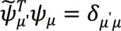 holds. At an EP, its left and right wave functions
  are also “self-orthogonal,” i.e., they satisfy
 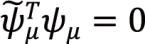 , while
 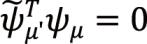 still holds when μ’ is different from μ. Therefore, if an inner product
 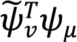 is finite, then two conditions must be satisfied: (1) ψμ is an eigenstate of H away from an EP, and (2) μ,v must be the same index. Since the inner product
 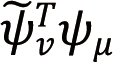 is finite for any right eigenstate ψμ of H, then none of the right eigenstates of H is at an EP, which indicates that H is not defective and has no EPs.
More importantly, with a positive-definite A and μ=ν, the first relation in Equation (3) then tells us that
$$ {\omega }_{\mu }={\omega }_{\mu }^{\ast }\in \mathbb{ℝ}\left(6\right)$$
for all ψμ’s, which concludes our proof that all energy levels of H are real and away from an EP when A is positive-definite.
If A is allowed to be positive semi-definite and have zero eigenvalue(s), we can still write A=B†B, but B now has zero eigenvalue(s). As a result, Equation (5) still holds but the equality cannot be eliminated, i.e., with Bψμ=0, and in turn, Aψμ=0, which violates the condition under which Equation (5) is derived. As a result, we find the following properties:
(1) If ψμ is an eigenstate of H with a non-zero eigenvalue ωμ, then Bψμ ≠0, and in turn, we find that ψμ is not at an EP and ωμ is real, similar to the case where A is positive-definite.
(2) Even if ψμ is an eigenstate of H with a zero eigenvalue, it is still not at an EP as long as Bψμ≠0.
(3) ψμ can be at an EP only if it is an eigenstate of B (and A, H) with a zero eigenvalue. In other words, H can only have an EP at ωμ=0, with the necessary condition that the corresponding eigenstate ψμ satisfies Aψμ=0.
In all our discussions above, the order of A and H0 in our construction of H is inconsequential; the other order AH0 gives H† with the same real eigenvalues.
To understand the conditions leading to the real spectrum of H in our construction, we focus on the special case where A is diagonal and H0 is given by a tight-binding model:
$$ {H}_{0}=\sum _{j}{\omega }_{j}|j⟩⟨j\left|+{t}_{j+1,j}\right|j+1⟩⟨j|+{t}_{j,j+1}|j⟩⟨j+1|,\left(7\right)$$
where ωj is the on-site potential and tj+1,j is the coupling from lattice site j to j + 1 and equals the coupling in the opposite direction, i.e., tj,j+1. By denoting the diagonal elements of A by aj’s, we first change the potential landscape, from ωj’s in H0 to aj ωj in H, which does not take place in an imaginary gauge transformation[21]. Although this procedure maintains the sign of the local potential, it can change a potential barrier to a well and vice versa. At the same time, we also scale the two couplings tj±1,j from site j by the same aj. This scaling, though, is direction dependent: the pair of couplings tj,j+1,tj+1,j between the two sites j, j +1 are scaled by aj+1,aj, respectively.
As an example, below we consider a one-dimensional system H0 with a harmonic potential[22]
$$ {\omega }_{j}={\left[j-\frac{N-1}{2}\right]}^{2}\frac{{\omega }^{2}}{2}(j={1,2},\dots ,N;N=100)\left(8\right)$$
(see Figure 1A) The coupling t∈ℝ is taken to be uniform. For the N eigenstates of H0, their lowest energies and corresponding wave functions follow closely the continuous case see Figure 1B and 1C, i.e.,
$$ {E}_{q}+2\left|t\right|\approx \left(q-1/2\right)\stackrel{~}{\omega },\left(9\right)$$
where q is a small positive integer. The offset 2|t| is due to the discrete nature of the system, and the effective natural frequency of the harmonic potential is given by 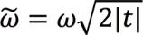 .
.
|
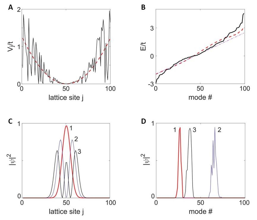
Figure 1. An Example of Constructing a non-Hermitian System with a Real Spectrum. A: Potential in H (solid) and H0 (dashed). ω2=t ∕1000; B: Spectra of H and H0, with that of the latter compared with the approximation given by Equation (9) (dash-dotted); C-D: Wave functions of the lowest three energy states in H0 and H, respectively.
Once we scale ωj (and t) by an arbitrary aj ∈ (0, 2] (see Figure 1A), the spectrum of H=H0A is very different and has a much longer tail at both the high and low end of the spectrum (see Figure 1B). Despite the asymmetric couplings in H, the wave functions of its eigenstates are still Anderson localized due to the random scaling we have introduced to the potential, especially the states near the two spectral ends where the spectral density is low (see Figure 1D).
Having exemplified our construction of a non-Hermitian Hamiltonian with a real spectrum, we note that the Hermitian Hamiltonian H0 in our construction of H cannot be replaced by a non-Hermitian matrix H′ with a real spectrum; the resulting H′′=H′A is not even pseudo-Hermitian in general.
One obvious exception is H′=A-1H0 where H0 is Hermitian, leading to a non-Hermitian H′′=A-1H0A with a real spectrum if A is non-unitary. This similar transformation from H0 to H, with A being diagonal and positive-definite, is the imaginary gauge transformation mentioned previously, which introduces a position-dependent scaling to the eigenstates of H0 and leads to the non-Hermitian skin effect[16,17].
The wave functions of H and H0 in our construction, on the other hand, are not simply related in general, and so are their (real) eigenvalues. This property, as it turns out, leads to a selective non-Hermitian skin effect: only the zero mode of the system, i.e., with ωμ=0, is exponentially localized at one edge of the system, while the non-zero modes remain in the bulk (Figure 2A). Here the original Hermitian H0 is given by the tight-binding model (7) with ωj=0 and tj,j+1=tj+1,j=t, and it has chiral symmetry that warrants the zero mode in both the Hermitian case (H0) and the non-Hermitian cases (H and H′′)[21]. Furthermore, one can show explicitly that the zero modes of H=H0A and H′′=A-1H0A are exactly the same (Figure 2), but they are formed by different mechanisms as we show below.
The standard non-Hermitian skin effect, as mentioned before, is caused by exponentiating the underlying Hermitian modes via a non-unitary transformation:
$$ {a}_{j}={s}^{j-1},{\psi }_{\mu ,j}^{{\text{'}}{\text{'}}}={\psi }_{\mu ,j}^{\left(0\right)}{s}^{-(j-1)},\left(10\right)$$
where j=1, 2,…,N and ψ′′μ,j, ψ(0)μ,j are the μth wave function of H′′,H 0 at site j, respectively. The skin modes are localized on the left (right) of the system when s>1 (0<s<1). The ratio of each pair of (nearest-neighbor) couplings is given by s2, and their geometric average remains unchanged as in H0 and uniform in space.
For the selective non-Hermitian skin mode in H, its formation is the combination of two effects. One is the same as the standard non-Hermitian skin effect but with the localization length doubled: the ratio of each pair of (nearest-neighbor) couplings is now given by s instead of s2, as can be easily checked. In the meanwhile, the geometric average of each pair (i.e., the effective coupling strength) also forms a geometric series, increasing by a factor of s from 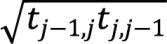 to
to 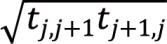 . This increment of the effective coupling strength, similar to the alternate strong and weak couplings in the Su-Schrieffer-Heeger (SSH) array[23] and the breathing Kagome lattice [24], contributes the same exponential factor to the wave function as the first mechanism. It then reduces the would-be localization length of the zero mode by half, and we recover the same zero-mode wave function given by Equation (10):
$$ {\psi }_{0,j}={\psi }_{0,j}^{\left(0\right)}{s}^{-(j-1)}.\left(11\right)$$
We also note that for the corresponding left eigenstate, each pair of couplings tj, j+1, tj+1, j are effectively exchanged, and hence the first mechanism alone would localize the left eigenstate on the right edge of the system instead, similar to what happens in the standard non-Hermitian skin effect (see the dashed line in Figure 2B). The second mechanism mentioned above is not affected by this exchange of tj, j+1, tj+1, j, because it is determined only by the geometric average of these two couplings. As a result, acting alone it would still localize the left eigenstate of the zero mode on the left edge of the system, and these two mechanisms hence cancel each other, causing the left eigenstate of the zero mode in the selective skin effect to be extended (see the dashed line in Figure 2A), which has the same spatial profile as the zero mode of the underlying Hermitian Hamiltonian H0.
|
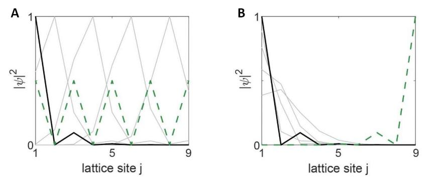
Figure 2. Comparison of Two Different non-Hermitian Skin Effects. A: Selective non-Hermitian skin effect; B: Standard non-Hermitian skin effect. Thick and thin lines show the zero and non-zero modes, respectively. Each thin line represents two modes related by chiral symmetry that have the same spatial profile. Dashed line in each panel shows the left eigenstate of its zero mode.
Also due to this increment of the effective coupling, the non-zero modes are now further away spectrally compared to those in H0 (and H′′). In the case shown in Figure 2A, the next two eigenstates of H are at ωμ=±2.38t, while those in H′′ shown in Figure 2B are at ωμ=±0.618t. Due to such energy differences, the wave functions of non-zero modes in H and H0 cannot be related directly, and the analysis leading to Equation (11) does not apply to them, indicating the absence of non-Hermitian skin effect in these modes. We also note that the onsite potentials ωj’s, which are scaled in H from H0 in general but not in H′′ as mentioned previously, do not play a role here because they are all zero.
Another difference between the selective and standard non-Hermitian skin effects is their vastly different lasing thresholds with a localized pump. In this consideration, each site in the tight-binding model represents a laser cavity, and it is typically a micro-ring or micro-disk laser by itself on an integrated photonic platform[25–27]. When the zero mode is the target lasing mode, intuitively one can pump the leftmost cavity in both systems, achieving the lowest lasing threshold by maximizing the spatial overlap between the pump and the zero mode[28].
In the tight-binding model, the radiation and material loss in each cavity are taken into account by making ωj complex, i.e., adding a negative imaginary part κ0. The pump compensates for this loss term by adding a positive imaginary part γj, and with spatially uniform pumping, all modes reach their non-interacting lasing threshold simultaneously, given by γj=κ0. Here the non-interacting thresholds ignore the competition for gain among the possible lasing modes, and the lowest one of all modes is the actual lasing threshold with modal interaction included in this framework, which is a simplified version of the semiclassical laser theory[2,3].
With the selective pumping scenario described above, however, only γ1 in the leftmost cavity is nonzero, and the threshold of the zero mode is the lowest in both H and H′′. Although the zero mode has the same spatial profile in these two cases, their thresholds still differ significantly. Denoting this zero-mode lasing threshold by D and D′′ in these two cases, they are given by D=1.44κ0 and D′′=4.99κ0 when the couplings are much stronger than the cavity loss (κ0=0.02t).
This difference is caused by the energy exchange between the system and the photonic environment at the coupling junctions[29], which can be quantified by analyzing the dynamical Equation (12) for the intensity in each cavity:
$$ \frac{d{\left|{\psi }_{j}\right|}^{2}}{dt}=2\left({\gamma }_{j}-{\kappa }_{0}\right){\left|{\psi }_{j}\right|}^{2}+{\mathcal{P}}_{j,j+1}+{\mathcal{P}}_{j,j-1}\left(12\right)$$
Where
$$ {\mathcal{P}}_{j,j+1}=i{t}_{j,j+1}^{\ast }{\psi }_{j+1}^{\ast }{\psi }_{j}+c.c.,{\mathcal{P}}_{j,j-1}=i{t}_{j,j-1}^{\ast }{\psi }_{j-1}^{\ast }{\psi }_{j}+c.c.\left(13\right)$$
are the inter-cavity power flows from cavity j+1 to j and from cavity j-1 to j respectively[29], and c.c. stands for the complex conjugation of the first term. This equation indicates that
$$ {\mathcal{G}}_{j,j+1}\equiv {\mathcal{P}}_{j,j+1}+{\mathcal{P}}_{j+1,j}=i\left({t}_{j,j+1}^{\ast }-{t}_{j+1,j}\right){\psi }_{j+1}^{\ast }{\psi }_{j}+c.c.\left(14\right)$$
is the power loss (if negative) or gain (if positive) at the coupling junction between cavities j and j + 1, which is non-zero only with asymmetric couplings (i.e., tj,j+1* ≠ t j+1,j).
Due to the non-Hermitian particle-hole (NHPH) symmetry of both H and H′′[30], the passive zero mode at γ1=0 becomes a non-Hermitian zero mode[31,32] as γ1 increases, i.e., without changing its frequency. Its spatial profile, however, is slightly perturbed from that shown in Figure 2, which is no longer “dark” with ψ0,j=0 at the even-numbered lattice sites (Figure 3A). This is another requirement for  j,j+1’s to be non-zero in the zero mode of both H and H′′, and their values are shown in Figure 3B. Clearly,
  j,j+1’s are all negative in both cases, indicating power loss at the coupling junctions. Furthermore, this power loss is one order of magnitude lower in H than H′′, leading to the much lower threshold in the former. This contrast becomes lower when the couplings are comparable to the cavity loss, e.g., we find D=1.35κ0 and D′′=1.62κ0 when κ0=t.
|
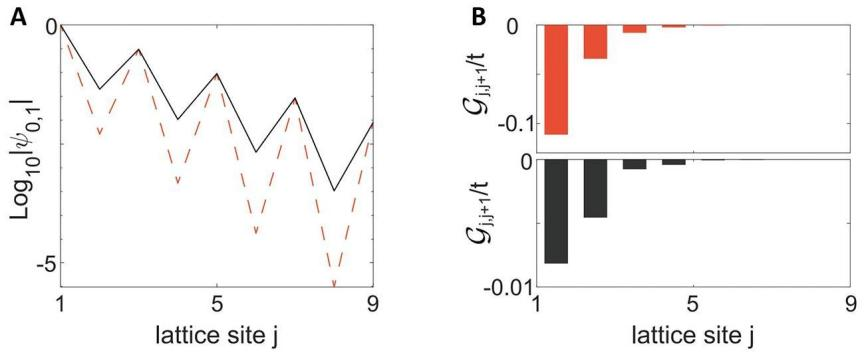
Figure 3. Analysis of the Lasing Mode at Threshold. A: Spatial profile of the zero mode at the lasing threshold in H (solid) and H′′ (dashed); B: Its loss to the photonic environment at coupling junctions in H (bottom) and H′′ (top).  j, j+1 is centered at j+1∕2 and with the normalization ψ0,1=1 in the leftmost cavity. Here κ0=0.02t.
4 DISCUSSION
So far, we have considered examples with a positive-definite A. If A has zero eigenvalue(s) (and is hence positive semi-definite), now H, still possessing a real spectrum, can have an EP at ωμ=0 as mentioned previously, if the corresponding eigenstate satisfies Aψμ=0.
As an example, we replace a4 by 0 in the diagonal A used in the case shown in Figure 2A. The resulting H has 6 real and non-zero real energy levels, paired by ωμ=-ων due to the chiral symmetry and NHPH symmetry. The other three eigenvalues are zero, but they do not form an EP of order 3. One of them is accompanied by the same selective skin mode ψ0 given by Equation (11), which is not an eigenstate of the modified A. Therefore, this eigenstate ψ0 cannot be at an EP of H as we explained earlier, and it forms a single-element Jordan block[33]. The other two zero eigenvalues form an EP of order 2 (EP2), with the coalesced eigenstate localized at j=4 (Figure 4B). This eigenstate, given by ψ0’ =[0, 0, 0, 1, 0, 0, 0, 0, 0]T, indeed satisfies Aψ0’ =0 as required. The location of this zero mode can be easily understood, because setting a4=0 means that the site j=4 does not couple to any other site, and the isolated wave function ψ0’ is guaranteed to be a zero mode. The corresponding Jordan chain that completes the Hilbert space can also be found analytically, i.e., HJ=ψ0’ with J=[-1, 0, s-2, 0, 0, 0, 0, 0, 0]T. The same outcome holds if we replace another aj by 0 instead, if j is even.
|
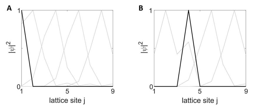
Figure 4. Zero Modes and EP. Both Panels are the same as Figure 2A, Except for A: With a1=0; B: With a4=0. Dashed line in B shows the zero mode at an EP2, while black solid lines in A and B show their zero mode not at an EP.
If this index is odd instead, the outcome becomes very different. For example, if we replace a1 by 0 instead, then ωμ=0 is non-degenerate and not an EP, and the isolated wave function is localized at the left boundary (Figure 4A), replacing the selective skin mode. In this case, the zero-mode wave function ψ0’ =[1, 0, 0, 0, 0, 0, 0, 0, 0]T again satisfies Aψ0’ =0, but as we mentioned previously, this latter condition is a necessary but not sufficient condition for ωμ=0 to be an EP of H.
Furthermore, if N is even instead that deprives H0 of a zero mode, now replacing one aj by 0 always gives rise to an EP2, independent of whether j is even or odd (not shown). This zero mode, localized at the jth site, again satisfies Aψ0’ =0 as required.
Another way to understand these results is the following. With a positive-definite or positive semi-definite, we write it again as B†B where B is an arbitrary square matrix. We then find
$$ \left(B{H}_{0}{B}^{†}\right)\left(B{\psi }_{\mu }\right)={\omega }_{\mu }\left(B{\psi }_{\mu }\right),\left(15\right)$$
which means:
If A is positive-definite, then B is of full rank. Therefore, B is invertible and H can be obtained by a similar transformation from the Hermitian Hamiltonian He≡BH0B†, i.e.,
$$ H={B}^{-1}{H}_{e}B,\left(16\right)$$
indicating that H has an entirely real spectrum. Furthermore, B provides an invertible mapping between the Hilbert spaces of He and H, which means every eigenstate φμ of He is mapped to a distinct eigenstate ψμ=B-1φμ of H, ruling out the possibility of having an EP.
When A (and B) is singular with zero eigenvalue(s), every eigenstate ψμ of H is mapped to an eigenstate φμ of He with the same eigenvalue ωμ, as long as Bψμ≠0. For a non-zero ωμ, Bψμ cannot be zero (it leads to ωμ=0), and hence these non-zero ωμ’s must be real, and so is the entire spectrum of H. At the same time, Heφμ=λμφμ leads to
$$ \left({B}^{†}B{H}_{0}\right)\left({B}^{†}{\phi }_{\mu }\right)={H}^{†}\left({B}^{†}{\phi }_{\mu }\right)={\lambda }_{\mu }\left({B}^{†}{\phi }_{\mu }\right),\left(17\right)$$
meaning every eigenstate φμ of He is mapped to an eigenstate of H† with the same eigenvalue λμ as long as B†φμ≠0. For a non-zero λμ, B†φμ cannot be zero (it leads to λμ=0). Using these observations and that H, H† have the same spectrum, we then arrive at the conclusion that the spectra of H and He are the same, but one cannot eliminate the possibility that H has EP(s).
As we mentioned in the introduction, our construction of a non-Hermitian H with a real spectrum can also be found in a system of coupled frictionless harmonic oscillators with different masses mi’s:
$$ {m}_{i}{\ddot{x}}_{i}=-2k{x}_{i}+k\left({x}_{i-1}+{x}_{i+1}\right).\left(18\right)$$
Here xi is the displacement of the ith mass, and all masses are connected sequentially by springs with the same spring constant k∈R. If we define the dynamical matrix M as
$$ \ddot{x}=Mx\left(19\right)$$
Where x=[x1,x2,…,xN]T , then M has the same form AM0 as in our construction, where A is a diagonal and positive-definite matrix with elements aj=mj-1 and M 0 is Hermitian and tri-diagonal, with -2k and k on its main diagonal and upper/lower diagonals. Clearly, the system is dissipationless and Hermitian, and hence the harmonic solutions x(t)=x(0)  have real-valued eigenfrequencies ωμ’s. Consequently, the eigenvalues of M, given by -ωμ2, are all real, despite that M is non-Hermitian if m i’s are different (e.g., M1,2=k ∕m1 ≠ M2,1*=k ∕m2).
We also stress that even when a non-Hermitian system has a real spectrum, it is our opinion that it should still be considered as a subsystem that exchanges particles and energy with its environment. Therefore, it is expected that the conservation of probability does not hold.
Nevertheless, there are other forms of generalized conservation laws that can be derived in non-Hermitian systems. One simple example is the conservation of probability or optical flux in a one-dimensional system. In a Hermitian system, this conservation law states that R+T=1, i.e., the summation of the reflected flux and the transmitted one is conserved. In a non-Hermitian PT-symmetric system, this conservation law evolves to  [34], where T is the still reciprocal transmittance from either the left or right side of the system which can now be larger than 1, while the reflectance from the left RL and that from the right RR can be different. In the Hermitian limit, T is always smaller than 1 and RR=RL≡R, and we recover R+T=1. Another example is the generalized Ehrenfest theorem defined with respect to a non-Hermitian inner product (A) ≡ψTAψ. When the linear operator A is not explicitly time-dependent, i.e. (dA/dt)=0, then it can be shown that (A) is a constant of motion when A defines a pseudo-chirality of the system, i.e., HT=-AHA-1[35].
5 CONCLUSION
In summary, we have presented a systematic approach to constructing non-Hermitian Hamiltonians with a real spectrum beyond a simple similar transformation, which can have embedded EPs at ωμ=0 depending on whether A has zero eigenvalue(s). A simple spectral shift can also realize an EP at any desired energy or frequency. Our approach utilizes the product of a Hermitian Hamiltonian H0 and a positive semi-definite matrix A. Despite bearing similarity to the polar decomposition of an arbitrary square matrix, i.e., as a product of a unitary matrix U and a positive semi-definite matrix A', here A and A' of H are different: A' is given by (H†H)1/2 = (AH02A)1/2 instead.
The positive semi-definite matrix A does not need to be diagonal, and when it is, we show that our approach can lead to a selective non-Hermitian skin effect, where the zero mode of the system is a skin mode while the non-zero modes still reside in the bulk. We have further shown that the formation of this selective non-Hermitian skin mode is due to two complement mechanisms, i.e., an imaginary gauge transformation and a non-uniform effective coupling strength, each contributing the same exponential factor to the localized spatial profile. Due to the reduced loss to the photonic environment at the non-reciprocal coupling junctions, the lasing threshold of this selective non-Hermitian skin mode is also much lower than its counterpart with the same spatial profile in the standard non-Hermitian skin effect, when we pump at the boundary where they are localized. Our approach may also find applications in constructing and understanding other non-Hermitian matrix operators, including but not limited to the coupled frictionless harmonic oscillators we have discussed.
This work is supported by the National Science Foundation (NSF) under Grants No. PHY-1847240 and No. DMR-2326698.
Conflicts of Interest
The author declares no competing interests.
Data Availability
All data generated or analyzed during this study are included in this published article.
Copyright Permissions
Copyright © 2024 The Author(s). Published by Innovation Forever Publishing Group Limited. This open-access article is licensed under a Creative Commons Attribution 4.0 International License (https://creativecommons.org/licenses/by/4.0), which permits unrestricted use, sharing, adaptation, distribution, and reproduction in any medium, provided the original work is properly cited.
Abbreviation List
PT, Parity-time
EP, Exceptional point
EP2, EP of order 2
References
[1] Gamow G. Zur quantentheorie des atomkernes. Z Phys, 1928; 51: 204-212.[DOI]
[2] Tureci HE, Ge L, Rotter S et al. Strong interactions in multimode random lasers. Science, 2008; 320: 643-646.[DOI]
[3] Ge L, Chong YD, Stone AD. Steady-state ab initio laser theory: generalizations and analytic results. Phys Rev A, 2010; 82: 063824.[DOI]
[4] Bender CM, Boettcher S. Real spectra in non-Hermitian Hamiltonians having P T symmetry. Phys Rev Lett, 1998; 80: 5243.[DOI]
[5] Mostafazadeh A. Pseudo-Hermiticity versus PT-symmetry. II. A complete characterization of non-Hermitian Hamiltonians with a real spectrum. J Math Phys, 2002; 43: 2814-2816.[DOI]
[6] Feng L, El-Ganainy R, Ge L. Non-Hermitian photonics based on parity-time symmetry. Nat Photonics, 2017; 11: 752-762.[DOI]
[7] Konotop VV, Yang J, Zezyulin DA. Nonlinear waves in PT-symmetric systems. Rev Mod Phys, 2016; 88: 035002.[DOI]
[8] Longhi S. Parity-time symmetry meets photonics: A new twist in non-Hermitian optics. EPL, 2018, 120: 64001.[DOI]
[9] Chen W, Kaya Özdemir Ş, Zhao G et al. Exceptional points enhance sensing in an optical microcavity. Nature, 2017, 548: 192-196.[DOI]
[10] Lai YH, Lu YK, Suh MG, et al. Observation of the exceptional-point-enhanced Sagnac effect. Nature, 2019; 576: 65-69.[DOI]
[11] Hodaei H, Hassan AU, Wittek S, et al. Enhanced sensitivity at higher-order exceptional points. Nature, 2017; 54: 187-191.[DOI]
[12] Rivero JHD, Feng L, Ge L. Imaginary gauge transformation in momentum space and Dirac exceptional point. Phys Rev Lett, 2022; 129: 243901.[DOI]
[13] Rivero JHD, Feng L, Ge L. Analysis of Dirac exceptional points and their isospectral Hermitian counterparts. Phys Rev B, 2023; 107: 104106.[DOI]
[14] Villegas-Martínez BM, Soto-Eguibar F, Hojman SA et al. Non-unitary transformation approach to PT dynamics. arXiv preprint arXiv: 201.06536, 2022.[DOI]
[15] Hatano N, Nelson DR. Localization transitions in non-Hermitian quantum mechanics. Phys Rev Lett, 1996;77: 570.[DOI]
[16] Hatano N, Nelson DR. Vortex pinning and non-Hermitian quantum mechanics. Phys Rev B, 1997; 56: 8651.[DOI]
[17] Gao Z, Qiao X, Pan M et al. Two-Dimensional Reconfigurable Non-Hermitian Gauged Laser Array. Phys Rev Lett, 2023; 130: 263801.[DOI]
[18] Zhang X, Tian Y, Jiang JH t al. Observation of higher-order non-Hermitian skin effect. Nat Commun, 2021; 12: 5377.[DOI]
[19] Wang W, Wang X, Ma G. Non-Hermitian morphing of topological modes. Nature, 2022; 08: 50-55.[DOI]
[20] Rivero JHD, Feng L, Ge L. Imaginary gauge transformation in momentum space and Dirac exceptional point. Phys Rev Lett, 2022; 129: 243901.[DOI]
[21] Rivero JHD, Feng L, Ge L. Analysis of Dirac exceptional points and their isospectral Hermitian counterparts. Phys Rev B, 2023; 107: 104106.[DOI]
[22] Leboeuf P, Moulieras S. Superfluid motion of light. Phys Rev lett, 2010; 105: 163904.[DOI]
[23] Su WP, Schrieffer JR, Heeger AJ. Solitons in polyacetylene. Phys Rev Lett, 1979; 42: 1698.
[24] Ezawa M. Higher-order topological insulators and semimetals on the breathing kagome and pyrochlore lattices. Phys Rev Lett, 2018; 120: 026801.[DOI]
[25] Chang RK, Campillo AJ. Optical Processes in Microcavities (Advanced Series in Applied Physics). World Scientific: Singapore, 1996.
[26] Vahala KJ, Optical Microcavities (Advanced Series in Applied Physics). World Scientific: Singapore, 2004.
[27] Cao H, Wiersig J. Dielectric microcavities: Model systems for wave chaos and non-Hermitian physics. Rev Mod Phys, 2015; 87: 61.[DOI]
[28] Ge L, Gao Z, Feng L. Non-Hermitian gauged laser arrays with localized excitations: Anomalous threshold and generalized principle of selective pumping. Phys Rev B, 2023; 108: 104111.[DOI]
[29] Ge L, Makris KG, Zhang L. Optical fluxes in coupled PT-symmetric photonic structures. Phys Rev A, 2017; 96: 023820.[DOI]
[30] Ge L. Symmetry-protected zero-mode laser with a tunable spatial profile. Phys Rev A, 2017; 95: 023812.[DOI]
[31] Qi B, Zhang L, Ge L. Defect states emerging from a non-Hermitian flatband of photonic zero modes. Phys Rev Lett, 2018; 120: 093901.[DOI]
[32] Ge L. Non-Hermitian lattices with a flat band and polynomial power increase. Photonics Res, 2018; 6: A10-A17.[DOI]
[33] Chen HZ, Liu T, Luan HY et al. Revealing the missing dimension at an exceptional point. Nat Phys, 2020; 16: 571-578.[DOI]
[34] Ge L, Chong YD, Stone AD. Conservation relations and anisotropic transmission resonances in one-dimensional PT-symmetric photonic heterostructures. Phys Rev A, 2012; 85: 023802.[DOI]
[35] Rivero JDH, Ge L. Pseudochirality: a manifestation of Noether’s theorem in non-Hermitian systems. Phys Rev Lett, 2020; 125: 083902.[DOI]
Brief of Corresponding Author(s)
Li Ge He received his PhD in Physics from Yale University in 2010, with his thesis focusing on laser physics in complex and disordered media, including wave-chaotic lasers and random lasers. He co-discoverered Coherent Perfect Absorbers. Before joining the City University of New York in 2013, professor Ge was a postdoctoral associate in the Department of Electrical Engineering at Princeton University. His current research interests include nonlinear and non-Hermitian phenomena in optics and photonics. Professor Ge has published more than 150 journal articles and conference proceedings in top scientific journals such as Science, Nature, Nature Physics, Nature Photonics, and Physical Review Letters, with a total citation over 10000 with an h-index of 43. |




 Copyright ©