Advanced Predictive Modeling for Hepatitis C Diagnosis Using Machine Learning

 

Mahdyeh Abbasi Hezari1, Marzieh Baes2*, Atyeh Abassi Hezari3, Mobina Hassanbabaei4

 

1Department of industrial Engineering, Faculty of Technology and Engineering, Alzahra University, Tehran, Iran

2Institute of Photogrammetry and GeoInformation, Leibniz Hannover University, Hannover, Germany

3Department of Bioelectric, Medical Engineering, Faculty of Medical Sciences and Technologies, Science and Research Branch, Islamic Azad University, Tehran, Iran

4Faculty of Psychology, Allameh Tabatabae’i University, Tehran, Iran

 

*Correspondence to: Marzieh Baes, PhD, Research Scientist, Institute of Photogrammetry and GeoInformation, Leibniz Hannover University, Nienburger Str. 1, Hannover, 30167, Germany; E-mail: baes@ipi.uni-hannover.de

 

DOI: 10.53964/cme.2024012

 

Abstract

The hepatitis C virus (HCV) virus, which has infected nearly fifty million individuals across the world, has recently been receiving significant attention. With the advent of artificial intelligence, there is an increasing effort to predict the HCV by utilizing machine learning models and training such models on relevant datasets. These data-driven models can aid doctors in the early detection of Hepatitis C infection. In this study, using datasets from the National Center for Health Statistics, we aim to develop a reliable model for predicting patients with positive hepatitis C tests. The most significant challenge in predicting such diseases using machine learning methods is finding an appropriate technique to address extremely imbalanced datasets, which arise from the smaller number of patients compared to healthy individuals in real-world datasets. We utilized real-world datasets and employed different machine learning algorithms, along with various methods for data balancing and feature selection. Unlike previous studies, which lacked this level of comprehensiveness, we utilized diverse feature selection and sampling methods such as Recursive Feature Elimination, Analysis of Variance (ANOVA) feature selection, Correlation matrix, synthetic minority over-sampling technique (SMOTE), BorderlineSMOTE, support vector machine synthetic minority over-sampling technique (SVMSMOTE), and Adaptive Synthetic Sampling (ADASYN) in conjunction with different machine learning algorithms including Random Forest, Decision Tree, XGBoost, AdaBoost, and logistic regression. We are the first to develop such a comprehensive study for the prediction of the HCV. Our findings suggest that we can predict patients infected by the HCV with a reasonable recall score of 0.86. This recall is achieved through the application of a model using the AdaBoost algorithm and the ADASYN method for balancing the dataset. The model's performance, especially on the validation dataset, was slightly better when we used ANOVA feature selection. Feature importance analysis conducted with ANOVA feature selection and Recursive Feature Elimination indicates that four to five features are the most prominent in our research analysis to predict patients with positive Hepatitis C tests.

 

Keywords: machine learning models, hepatitis C, imbalanced dataset, prediction

 

1 INTRODUCTION

The liver, as the largest internal organ in the human body, plays a vital role in detoxifying different substances and removing waste products from the body. It processes and filters toxic substances, drugs, alcohol, and harmful substances and converts them into less harmful products that can be excreted by the kidneys or intestines. Due to various factors such as poor and unhealthy lifestyles, a considerable percentage of the world’s population is at risk of developing liver diseases. According to the World Health Organization (WHO), hepatitis C virus (HCV) infection, one of liver diseases, has affected nearly 58 million individuals in the world. Since there is currently no effective vaccine against HCV, early diagnosing is a crucial step in controlling the disease.

 

The continuous advancement in mathematical modeling, particularly in the modeling with fractional calculus has shed light on the dynamics of various infections and has provided powerful tools to study the spread and control of diseases like pertussis, dengue, chikungunya, monkeypox, and HIV[1-6]. Building on this trend of utilizing advanced mathematical techniques, our study will use ML models to analyze and predict HCV from simple datasets such as demographic data and blood tests. ML models, as opposed to traditional mathematical modeling which needs complex mathematical formulations, provide us with sophisticated predictive models by a straightforward method that involves extracting patterns and relationships from data. Building ML models can be a big step towards timely diagnosis and treatment, which reduces the risk of serious complications such as cirrhosis and liver cancer, saving thousands of human lives each year.

 

Several studies have been conducted to investigate HCV using artificial intelligence methods. Zdrodowska et al.[7] used a dataset containing information of 73 patients with three classes of HCV (a) without or with minor fibrosis, (b) with fibrosis, and (c) end-stage liver cirrhosis. The authors utilized four ML algorithms of Naive Bayes, J48, Support Vector Machine (SVM), and random fores tand two feature selection methods of Gain Ratio Attribute Evaluation and Info Gain Attribute Evaluation to predict these three classes. Their best model, which was based on the SVM algorithm correctly classified 75% of instances. Minami et al.[8] built an application to predict hepatocellular carcinoma development after the eradication of HCV with antivirals. They used data from 1,742 patients with chronic HCV who achieved a sustained virologic response. Five ML methods of DeepSurv, Gradient Boosting Survival, Random Survival Forest, Survival SVM, and Conventional Cox Proportional Hazard were used among which Random Survival Forest resulted in the best model performance. Ali et al.[9] used attenuated total reflection Fourier transform infrared spectroscopy to predict hepatocellular carcinoma development in patients infected by HCV. They utilized freeze-dried sera samples collected from 31 HCV-related hepatocellular carcinoma patients and 30 healthy individuals. Their model results showed an accuracy of 86.21% for the classification of the non-angio-invasive hepatocellular carcinoma/angio-invasive hepatocellular carcinoma status.

 

Ahn et al.[10] focused on developing a data-driven model that was able to distinguish between patients with acute cholangitis (AC) from individuals with alcohol-associated hepatitis (AH) based on several laboratory parameters that were easy to interpret. The dataset consisted of 459 observations, including 265 from AH and 194 from AC. In total, eight ML algorithms were utilized: Decision Tree, Naive Bayes, logistic regression, K-Nearest Neighbour, SVM, Artificial Neural Networks, Random Forest, and Gradient Boosting. A single feature selection strategy was utilized to select most important features. The authors indicated that their best model could achieve an accuracy of 0.932 and an area under the curve (AUC) of 0.986. Using a feature selection method they could further improve the model performance. Park et al.[11] trained Multivariable logistic regression, Elastic Net, Random Forest, Gradient Boosting, and Feedforward Neural Network ML models to predict direct-acting antiviral treatment failure among patients with HCV infection. They analyzed a total of 6,525 samples. Their best model was the Gradient Boosting model, with a recall of 66.2%. Farghaly et al.[12] utilized a dataset with 859 samples that included 11 different features. They modeled HCV, using Naive Bayes, Random Forest, K-Nearest Neighbor, and logistic regression. In addition, they used the sequential forward selection-based wrapper feature selection. The outcomes of this study revealed that the random forest model was the best at predicting HCV, with 94.88% accuracy and a recall of 84.52%. Kim et al.[13] employed National Health and Nutrition Examination Survey (NHANES) data from 2013-2018 to build a model predicting HCV and Hepatitis B Virus (HBV) among diabetic patients. Their datasets included 1,396 diabetic samples with mean age of 54.66 years, among which 64 samples were those infected by HBV or HCV and 1,332 records were without HBV or HCV infection. They built several models including random forest, SVM, XGBoost, least absolute shrinkage and selection operator (LASSO), and stacked ensemble model. To mitigate the unequal sample problem among the different classes, authors used the SMOTE method. They concluded that the LASSO model was the best performer with a classification AUC-ROC of 0.810. Lilhore et al.[14] employed a workflow that included sampling using SMOTE, feature selection, and a hybrid predictive model using a random forest improved algorithm and SVM to predict HCV. They used a dataset with 1,756 records, consisting of 1,056 unhealthy and 700 healthy samples. Their model demonstrated an accuracy of 41.541% (recall score of 40.55%) without SMOTE and 96.82% (recall score of 99.13%) with Synthetic Minority Over-sampling Technique (SMOTE).

 

1.1 Originality and Innovations Compared to Previous Works

To our knowledge, no studies predicting HCV have employed a comprehensive approach combining various sampling methods and feature selection techniques to train models on real-world datasets. One of the main limitations of some past studies is the use of an improper metric. For instance, accuracy is not an appropriate metric when the data classes are imbalanced as it mainly evaluates the model performance on the majority class. Another limitation in some studies is the dataset size. Limited sample size restricts the model’s ability to generalize, as increasing the number of data samples typically enhances the model’s generalizability to new, unseen data. Moreover, selecting appropriate samples with a realistic distribution of healthy and unhealthy samples is another missing point in some previous studies. In the real world, the number of patients infected with HCV is much smaller than that of healthy individuals. Another limitation in many studies was the absence of using complementary methods, such as various feature selection and sampling techniques, to improve model performance. Since sampling of minority classes and eliminating irrelevant features can significantly enhance model performance and simplify model application, it is essential to explore models with different sampling and feature selection methods to achieve optimal performance.

 

In this study, we specifically aim to address and overcome several of the limitations identified in previous studies. Using five distinct ML models (logistic regression, decision tree, random forest, AdaBoost, and XGBoost), we explore the impact of various sampling methods (SMOTE, BorderlineSMOTE, support vector machine synthetic minority over-sampling technique (SVMSMOTE), and Adaptive Synthetic Sampling (ADASYN)) and feature selection approaches (correlation matrix, Recursive Feature Elimination and Analysis of Variance (ANOVA) feature selection) on model performance. Moreover, we utilize real-world datasets of NHANES, which strengthens our work in a thorough and data-informed manner. In this study, we develop and assess 40 different models to determine the best predictive model for HCV. The aim is to provide a rigorous and generalizable framework which addresses the challenges of imbalanced data and limited sample sizes often encountered in previous studies. This paper is structured as follows: we first describe the dataset used in this study. Next, we explain the methods including data preparation, ML algorithms, feature selection techniques, sampling methods utilized in this study, and hyperparameter tuning. We then detail the model-building process. Finally, we present and discuss the model results and draw our conclusions.

 

2 DATASET

In this study, we used open datasets from the National Center for Health Statistics (NCHS), which is a division of the Centers for Disease Control and Prevention (CDC) under the United States Department of Health and Human Services (HHS). The NCHS is responsible for collecting health data using different methods such as surveys and administrative data systems. Among its other responsibilities are analyzing and publicizing data on its website to be accessible worldwide. The main characteristics of the data provided by NCHS are their high accuracy, integrity, and objectivity.

 

Here, we focused on NHANES datasets, which are publicly available and anonymized. The use of these datasets complies with all ethical guidelines, as the data is de-identified and poses no risk to individual privacy. We used demographic, physical examination results, and laboratory data spanning the years 2005 to 2020. The NCHS typically releases these datasets in two-year cycles, except for the years 2017-2020, which were issued as combined datasets spanning three years. These datasets are available via multiple files to enrich accessibility and usability. After extracting, merging, and cleaning the datasets from the NCHS website, we obtained a dataset with a total of 10,818 data points. Among these data, there were only 197 positive HCV test samples, highlighting an extremely imbalanced dataset. Addressing this imbalance was a critical step in our analysis.

 

3 METHODS

To classify and predict patients infected with HCV, we have tested several ML algorithms. Due to the fact that the number of HCV-infected individuals is much smaller than that of uninfected ones, we have applied some techniques to deal with the highly imbalanced data. We have also applied some feature selection techniques to remove non-essential features, leading to an improvement in model performance and a reduction of computation time. Following is a brief description of data preparation, the techniques used to address the imbalanced dataset, followed by descriptions of the ML algorithms, feature selection methods employed in this study, and hyperparameter tuning.

 

3.1 Data Preparation and Exploratory Data Analysis (EDA)

The dataset used in this study was obtained from the website of NCHS. The original data were stored in the format of XPT, which stands for statistical analysis system transport file. In the first step, we converted the format of datasets from XPT to Comma Separated Value (CSV), which is a user-friendly and easy-to-use format. Next, we explored and analyzed the datasets. The datasets included three classes of positive, negative, and negative screening HCV Antibody. We merged the negative and negative screening HCV Antibody classes into a single negative class. The resulting datasets were highly imbalanced two-class datasets. To address the missing values in highly imbalanced datasets, we imputed them by using the mean of each feature within its respective class. In the next step, we merged all the datasets from different years. Then, we applied a logarithmic transformation to scale the data and transfer them to a nearly normal distribution. Subsequently, by analyzing the correlation matrix, we removed two features that were highly correlated with other features. A more detailed description of the EDA process will be discussed later in the “ML models” section. 

 

3.2 Strategies for Handling Imbalanced Datasets

Classification problems are highly dependent on having a nearly balanced dataset. In imbalanced datasets, accuracy represents the evaluation of model performance in predicting the majority class. In such cases, when an appropriate metric that reflects model performance in classifying the minority class (for instance F1-score or Recall) is used, it becomes evident that the model performance for predicting the minority class is poor. Since the number of samples in the minority class is low, the model cannot capture the patterns within the minority class data effectively. Therefore, it is essential to balance data before training the models. Since our dataset is highly imbalanced, we employed the following methods:

 

3.2.1 SMOTE

Oversampling the minority class instances is one of the methods to address the problem of imbalance datasets. There are numerous methods to oversample instances of the minority class. The most straightforward way, which leads to balance in distribution, is to duplicate existing samples from the minority class. Duplication does not, however, add any new information to the model. A more sophisticated method of oversampling the minority class appears to involve the synthesizing of new examples from the minority class. SMOTE is one of the common means of synthesizing new examples by selecting instances that are close together in the feature space and generating new samples from minority class instances by interpolation[15,16]. In this approach, a synthetic sample of a given feature is created by interpolation between a randomly selected instance from the minority class and one or more of its neighbors. Balancing classes by sampling of minority instances reduces bias caused by the imbalanced data which leads to an improvement in the performance of ML models.

 

3.2.2 BorderlineSMOTE

BorderlineSMOTE as an extension of SMOTE is the one that deals with the borderlines of the minority class. Borderlines are the areas near the dividing lines between the minority and majority classes where the probability of errors made by the model is high. BorderlineSMOTE is a model that uses SMOTE to synthesize new observations of the minority class near the boundary between the two classes[17]. In this model, the borderline samples are identified by KNN (K-Nearest Neighbors) approach.

 

3.2.3 SVMSMOTE

Another extension of SMOTE is SVMSMOTE, which integrates the principles of SMOTE with SVM to produce synthetic samples for the minority class[18]. Like BorderlineSMOTE, SVMSMOTE focuses on borderline instances in the minority class. It uses support vectors, which are data points located close to the decision boundary between different classes, for synthetic sample generation. This is in contrast to BorderlineSMOTE in which the KNN (K-Nearest Neighbors) method is used to identify borderline instances.

 

3.2.4 ADASYN

Similar to SMOTE, the ADASYN has been invented to overcome the issue of class imbalance by producing simulated examples for the minority class. In this method, the generation of synthetic samples is carried out adaptively, which means that the method adjusts itself according to the areas that are difficult to learn in the feature space. This is in contrast to SMOTE, which produces synthetic samples uniformly. ADASYN generates more synthetic data for minority instances that are harder to classify. Consequently, it enhances model performance by reducing the bias originating from class imbalance and dynamically adjusting the classification decision boundary towards challenging instances[19].

 

3.3 ML Algorithms

Artificial Intelligence approaches have been heavily exploited in the development of data-driven models. ML as a part of AI, has numerous applications across multiple domains such as environmental science, social sciences, business, and life sciences. ML models are based on analyzing the data and recognizing patterns within it. These models in turn can be employed as predictive means.

 

In this study, five supervised ML algorithms were used to predict patients infected with HCV. Supervised ML algorithms work on labeled data. At first, patterns and relationships in labeled training datasets are learned by the model. After the training, the model will predict or make decisions on new unknown unlabeled datasets. Below, we provide a brief explanation of the algorithms used in this paper.

 

3.3.1 Logistic Regression

Logistic regression is a supervised learning algorithm that is based on statistical methods, capable of predicting binary processes. Its algorithm is based on estimating the probability of a sample falling into a particular class. The logistic regression algorithm is like the linear regression method that models the dataset by fitting a line to it. However, instead of fitting a line, logistic regression uses a sigmoid function (which maps any number into a number between 0 and 1) to predict the relationship between the independent (features) and the binary dependent (target) variables[20]. The main difference between linear and logistic regression methods is in their applications: linear regression is used in regression problems (for predicting continuous values) while logistic regression is utilized in classification problems. It is noteworthy to mention that logistic regression behaves inadequately when the classes are heavily imbalanced. Therefore, it is important to balance the datasets when using this algorithm.

 

3.3.2 Decision Tree Classification

Decision tree is another powerful widely-used ML method. The decision tree structure resembles a tree with a root node and its branches that are expanded into further branches[21]. Decision tree relies solely on binary responses to simple yes or no questions to arrive at an outcome. The algorithm mimics our own thinking ability, which can lead to easy conceptualization. The decision tree can be used for both classification and regression problems. The major disadvantage of the decision tree is its tendency to overfitting (performing well on the training dataset but poorly on a new dataset), particularly in models composed of deep trees or through noise in the dataset. If overfitting occurs, there are several methods to overcome this problem. For instance, constraining the maximum depth or using a bagging method (for instance an ensemble technique) can help resolve the problem of overfitting.

 

3.3.3 Random Rorest Classification

Another extremely popular supervised ML algorithm is the random forest algorithm. The random forest algorithm can be developed for both classification and regression problems. As the name suggests, the random forest is based on developing multiple decision trees to assist in resolving complex problems[22].

 

Random forest is an ensemble learning method that combats complex problems by taking multiple classifiers/regressors and combining them for a definitive outcome. It relies on the bagging technique which splits the dataset into ‘n’ number of subsets. The decision trees are then constructed on each of these ‘n’ subsets. In other words, random forest is based on constructing multiple models independently on different subsets of data (bagging) that results in a robust model for overcoming the overfitting problem.

 

3.3.4 AdaBoost Classification

AdaBoost, short for Adaptive Boosting, is another ensemble learning technique used for both classification and regression tasks. It is based on the Boosting method in which a sequence of weak classifiers is iteratively trained on different subsets of the data[23]. In each iteration, weights are assigned to the samples to ensure that the samples that were misclassified in the previous iteration are given higher weights. In other words, the misclassified samples are prioritized such that the next weak classifier improves model performance.

 

3.3.5 XGBoost Classification

Extreme Gradient Boosting or XGBoost, builds and combines decision trees using a Gradient Boosting approach. It has been widely used in countless ML tasks, both in regression and classification problems[24]. XGBoost, like AdaBoost, uses a Boosting method that builds a prediction model from consecutive weak predictors. The model focuses on those instances with higher weight assignments - these instances were classified poorly in the previous iteration. By focusing more on instances with higher weights, model performance improves. The training procedure is based on maximizing differentiable loss functions.

 

3.4 Feature Selection

In an ML task, we often deal with large datasets containing various features. Incorporating some of these features into the model training might make the predictions worse. Besides, the contribution of some features to the model training might be negligible, however, their inclusion in the model is computationally expensive. Thus, feature selection is a critical step in creating ML models through the recognition of the most significant and relevant features. The primary benefits of using feature selection are the improvement of the performance of the ML model and computational savings. There are many methods for feature selection, and here, we used three of them, which are the correlation matrix, recursive feature elimination (RFE), and ANOVA feature selection.

 

3.4.1 Correlation Matrix

The correlation, which measures the linear relationship of a pair of features in the dataset, is one of the popularly used feature selection methods, especially when there is a linear relationship between the features[25,26]. The correlation matrix indicates how strongly and in which direction two features are related. By calculating pairwise correlations between features, we can assess which features are highly correlated with the target variable and with each other. The presence of a feature with a weak relationship with the target variable in the model reduces the impact of some potentially important features. Besides, the inclusion of features that are highly correlated with each other, adds computational complexities to the model, without improving model performance. Therefore, eliminating features that are highly correlated with each other or have a poor relationship with the target may improve model performance.

 

3.4.2 RFE

RFE is a feature selection approach that is based on removing features sequentially until it reaches the number of desired features[27,28]. It utilizes the backward selection method to establish an ideal combination of features. In this process, first, the model is trained on all features and then the importance score for each variable is evaluated and the feature with the least importance is removed. This process is repeated until the number of desired features is reached. Then the model is trained and run with only the important features again. The number of desired features is assumed to be known in RFE, which can either be obtained from other sources, for instance from previous modeling systems/studies, or through hyperparameter tuning. In this study, we obtain the number of desired features by considering it as a model hyperparameter, which is tuned before model training. 

 

3.4.3 ANOVA Feature Selection

Another feature selection method used in this study is the ANOVA ranking scheme, which is based on a statistical test called the F-test. In this approach, features are ranked through the ratio of variances between groups and within groups[29]. After the ranking of features, we then remove low-ranked features. Since one of the assumptions in the F-test is that the data is normally distributed, we must account for a dataset that is close to a normally distributed dataset.

 

3.5 Hyperparameter Tunning

hyperparameters are parameters that control the learning process and must be set before model training. The principal difference between hyperparameters and parameters of the model is that hyperparameters are tuned prior to training, while parameters of the model are the end results of the ML process. hyperparameter tuning is critical in any ML model; the correct hyperparameter tuning could drastically improve the model, while the incorrect hyperparameter tuning may cause underfitting (performing poorly on both training and validation data) or overfitting of the model. The goal is always to find the hyperparameters leading to the best model performance on both the training and validation datasets.

 

There are various ways to tune hyperparameters including grid search, random search, and Bayesian optimization. In this work, we utilize random search, which is based on random sampling from various combinations of hype-parameter values within a specified range. The performance of hyperparameter tuning is evaluated by K-fold cross-validation, where the dataset is divided into K folders with K-1 training folders and one validation set.

 

4 ML MODELS

As indicated earlier, a total of 10,818 samples from the NHANES dataset were used to develop a data-driven model for HCV prediction. Figure 1 shows the workflow that we followed in this study. The first step was to select the datasets and their features from the NHANES website. Datasets spanning from 2005 to 2020 with 25 features were chosen (Table 1). After data extraction and preparation, we conducted an Exploratory Data Analysis (EDA) to analyze the dataset. Missing values for each feature were imputed using the mean of that feature within its respective class.

 

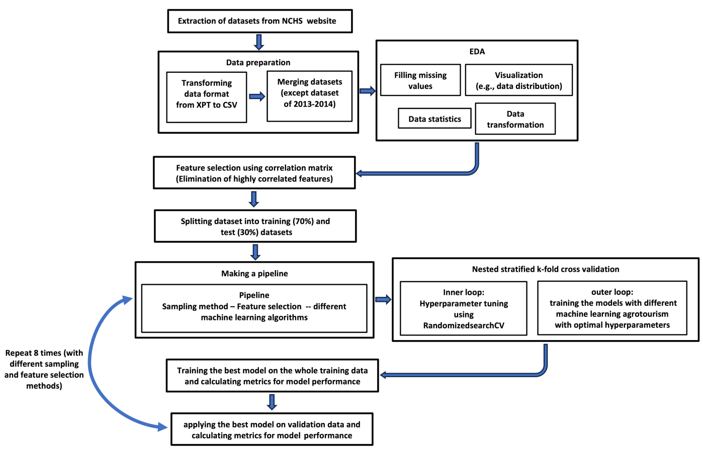
Figure 1. The Workflow used in this Study which Includes Several Key Stages: Data Preparation, EDA, Feature Selection, Data Splitting, and Model Training and Validation. A detailed explanation of this workflow is provided in the ‘ML models’ section of the text.

 

Table 1. Features Used in ML Models

 

Next, we explored the statistical distribution of features. The data distribution of most of the features showed a right-skewed distribution. To make the data distributions more symmetric and normal-like, we used a logarithmic transformation. By doing this transformation,  the distribution of most of the features became nearly normal (Figure 2) which is a favorable condition for certain ML algorithms like linear regression, and logistic regression. Besides, logarithmic transformation results in data scaling, which is one of the essential steps in any ML models. In the next step, we eliminated features with high correlation using a correlation matrix which indicates how two features correlate. The correlation matrix showed that there were high correlations between LDL cholesterol and total cholesterol as well as waist circumference and BMI (Figure 3). To avoid unnecessary complexity of the model and help in speeding up computations, we eliminated LDL cholesterol and waist circumference features.

 

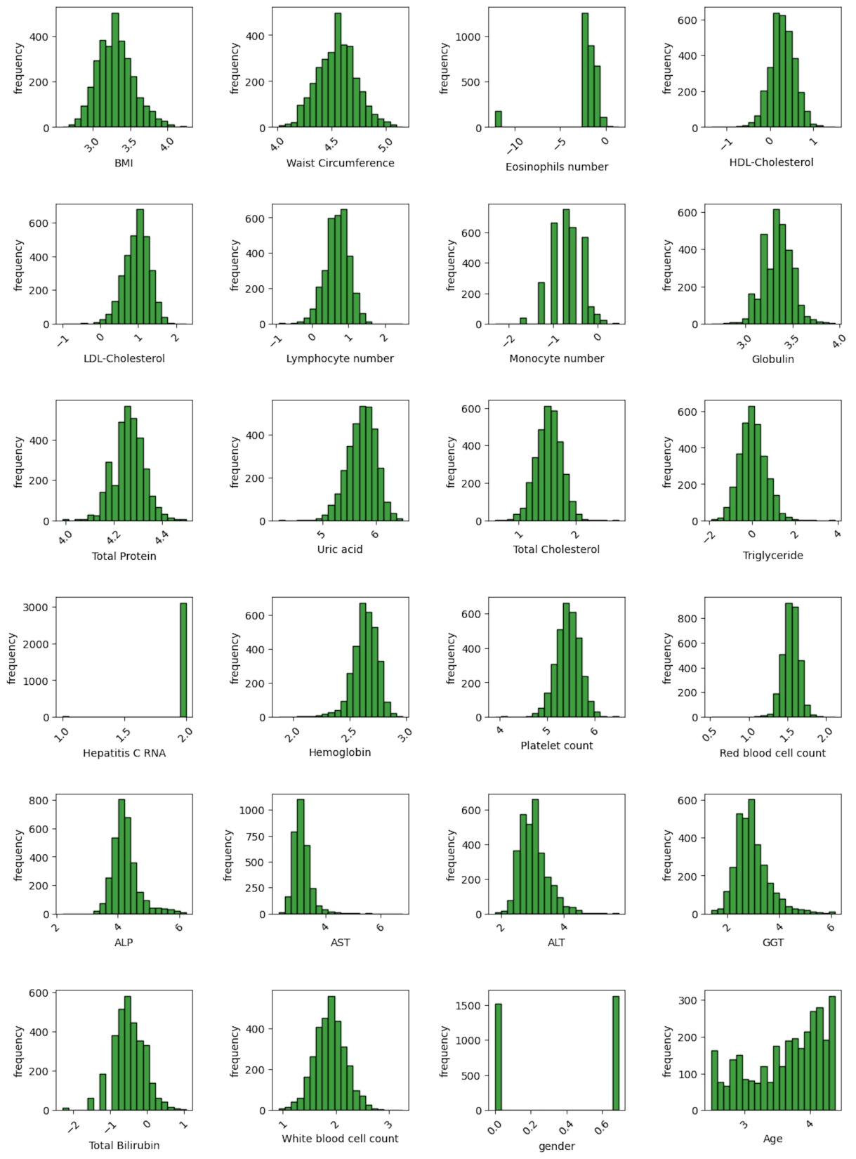
Figure 2. Data Distribution of Features After Applying Logarithmic Transformation. The distribution of most features is close to a normal distribution.

 

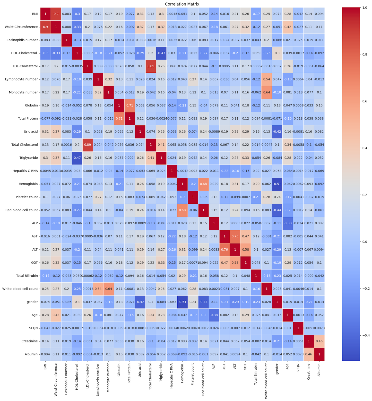
Figure 3. Correlation Matrix. The matrix shows that BMI and total cholesterol are highly correlated with waist circumference and LDL cholesterol, respectively, which may not be favorable for some ML algorithms.

 

In the next step, the dataset was divided into three subsets: train, test, and validation. The training dataset, which was used for training the models to capture the main pattern of the data, was considered to be 70% of the total dataset (excluding the dataset of years 2013-2014 which was considered as the validation dataset). The remaining 30% of the data was utilized to test the performance of the models. The validation dataset, which was the dataset of years 2013-2014, was used to assess model performance on new, unseen datasets. Due to the highly imbalanced dataset, we divided the dataset into test and train data using stratified sampling, in which the samples are selected in the same proportion concerning the number of majority and minority instances. This guarantees that minority class samples are available in both test and train datasets.

 

To implement the sampling methods, feature selection technique, and ML algorithms, we built a pipeline using the pipeline library in Python. Our pipeline includes one sampling method, one feature selection technique, and five ML algorithms. For each sampling and feature selection method we developed a new pipeline (we repeated the stages of building a pipeline till the evaluation of the model in Figure 1 eight times to include different sampling (four methods) and feature selection (two methods) techniques). In each pipeline, the first step is to balance the imbalanced dataset by adding synthetic samples to the minority class, using a sampling method. Then, relevant features were selected by evaluating the feature importance scores after building an ML model. Since training the model only on one training dataset and evaluating the result with test data does not usually guarantee the reliability of model performance on new and unseen datasets, we used stratified K-fold cross-validation[30] to evaluate the generalization of the model. In stratified K-fold cross-validation, the training dataset is divided into K subsets and the model is trained K times. Each time, K-1 subsets are used as training data and one subset is considered as the test data. In this way, the model results are more robust as the model is trained and evaluated multiple times on unseen datasets. Since our dataset is imbalanced, we used stratified K-fold cross-validation, where the training data is split into K subsets such that the proportion of each class is preserved in each subset. To simultaneously tune hyperparameters, we employed nested stratified K-fold cross-validation, a method used to evaluate model performance and concurrently optimize its hyperparameters. In nested stratified K-fold cross-validation, hyperparameters are tuned in the inner loop by examining different hyperparameter configurations. In the outer loop, the model performance is evaluated. In this study, we used 10-fold cross-validation for inner and outer loops. This means that in each loop the data was divided into 10 subsets and each subset served as the validation set once, while the remaining 90% was used for training. While 10-fold cross-validation can improve model performance, it is computationally expensive, which is one of the limitations of using large values for K in the K-fold cross-validation process. For tuning hyperparameters, there are various methods for selecting different combinations of hyperparameters. Here, we used random search[31], which randomly samples a fixed number of parameter settings from specified hyperparameters. Table 2 lists the hyperparameters that were tuned in our study including hyperparameters of ML algorithms, the number of desired features, and hyperparameters of sampling techniques along with their specified ranges of values.

 

Table 2. hyperparameters for Different ML Models, Feature Selection Approaches, and Sampling Techniques Used in This Study Along with Their Value Ranges

 

To better evaluate the performance of models, we plotted learning curves for each of our models. The plot of learning curves, which shows how well a model learns from the data and how well it generalizes to new and unseen data, is a great tool for evaluating model performance and identifying overfitting or underfitting. We also applied the best ML model to the 2013-2014 validation dataset to assess its robustness and generalizability.

 

5 MODEL RESULTS AND DISSCUSION

In this study, we developed ML models using decision tree, random forest, XGBoost, AdaBoost, and logistic regression algorithms. We conducted a total of 40 ML models with a combination of various ML algorithms, feature selection approaches, and sampling techniques. Table 3 summarizes the results of different models. We assessed the performance of our models with multiple metrics such as accuracy, precision, recall, F1-score, and confusion matrix. A confusion matrix can be defined as a table that allows a classification model's performance to be effectively summarized by displaying the number of true positives (TP), true negatives (TN), false positives (FP), and false negatives (FN):

	Predicted Positive	Predicted Negative
Actual Positive	True Positive (TP)	False Negative (FN)
Actual Negative	False Positive (FP)	True Negative (TN)

 

Accuracy, precision, recall and F1-score are defined as:

$$ Accuracy=\frac{TP+TN}{TP+FP+TN+FN}$$

$$ Precision=\frac{TP}{TP+FP}$$

$$ Recall=\frac{TP}{TP+FN}$$

$$ F1-score=2\times \frac{Precision\times Recall}{Precision+Recall}$$

 

It is noteworthy to indicate that in this study, the best model was evaluated based on recall scores of the minority class. This is because our aim here is to develop a model with a minimum error in predicting patients with positive HCV, meaning a model with a minimum number of FN. Recall score is a relevant metric where misclassification of positive instances (FN) has a high cost. The recall scores of the minority class in our models range from 0.53 to 0.86, with FN number of 23 and 7, respectively. The best model performance with a recall score of 0.86 and 7 False Negatives was achieved when we used the AdaBoost classifier in combination with ADASYN sampling, regardless of the feature selection methods (models M11 and M12 in Table 3). XGBoost models with different sampling methods and feature selection techniques gave poor results in the prediction of minority class in our study. However, the best accuracy scores are related to XGBoost, random forest, and logistic regression models with the SVCSMOTE sampling method (models M25-M30). This reveals that these models perform well in predicting healthy individuals (Negative samples) which are the majority, confirming that the accuracy score is not a suitable metric in models dealing with a highly imbalanced dataset.

 

As seen in Table 3,random forest models nearly always perform well in predicting negative samples when employing different sampling and feature selection methods. This indicates the robustness and ability of the random forest algorithm in prediction, especially when the data is almost balanced. The numbers of incorrectly classified negative samples of our best models (models M11 and M12), in which the AdaBoost algorithm and ADASYN sampling method were used, are 289 and 368 for RFE and ANOVA feature selection techniques, respectively. Results of models like random forest and XGBoost show a better prediction for negative examples, however, here we aim to minimize error in predicting positive samples since the cost of prediction error for positive samples is high. There is no risk in misclassifying healthy individuals. The only consequence of this misclassification is taking a follow-up HCV test. However, errors in positive samples’ prediction can delay the treatment process which may result in the further development of disease and threaten the life of patients.

 

Table 3. Model Results of Different ML Algorithms, Sampling and Feature Selections Techniques

Notes: The table includes the classification report (precision, recall, and F1-score), confusion matrix, and recall of the minority class. For a detailed explanation of the precision, recall, F1-score, accuracy and confusion matrix, please refer to ‘Model results and discussion’ section of the text.

 

Based on our results from models using various sampling and feature selection methods, the ADASYN sampling technique consistently enhances model performance in predicting positive samples across almost all algorithms (M11-M20). In contrast, while other sampling methods enhanced model performance with certain algorithms, they did not consistently improve performance for all models. This emphasizes the strengths of ADASYN and its applicability for producing trustworthy predictive models across various algorithms.

 

Across various ML algorithms, SMOTE showed better model performance compared to SVCSMOTE and BorderlineSMOTE, while SVCSMOTE demonstrated the lowest model performance. The best model performance for ADASYN, SMOTE, SVCSMOTE, and BorderlineSMOTE was achieved when we used AdaBoost, logistic regression, AdaBoost, and decision tree, respectively (Table 3). These outcomes illustrate how important it is to use the correct sampling method for different algorithms when dealing with highly imbalanced datasets. Comparing different feature selection methods, we found that the ANOVA feature selection gave slightly better model performance than RFE, and this was more apparent when we evaluated our best model on the validation dataset, where the recall score increased from 0.77 to 0.89 (Table 4).

 

Table 4. Evaluation of the Performance of the Best Model on Validation (New and Unseen) Dataset

Notes: The table includes the classification report (precision, recall, and F1-score), confusion matrix, and recall of the minority class. For a detailed explanation of the precision, recall, F1-score, accuracy and confusion matrix, please refer to ‘Model results and discussion’ section of the text.

 

Table 5 compares our study with those of Farghaly et al.[12] and Lilhore et al.[14], which are two studies similar to the current one. The contents of this table clearly demonstrate the comprehensiveness and excellent performance of our model. Our best model recall score is better than the recall score of models in Farghaly et al.[12]. However, it is slightly lower than that in Lilhore et al.[14]. The reason for the lower recall score in our study compared to Lilhore et al.[14] can be attributed to the nature of the datasets. In our study, the number of samples in the minority class (people affected by HCV) is 1.82% of the total number of samples while in Lilhore et al.[14] it is 39.86%. This difference indeed reflects our choice of real-world datasets and the challenge of training a model on a highly imbalanced dataset. Considering the percentage of imbalanced data, our approach to tackling the problem of imbalanced datasets is unique and satisfactory. Noteworthy to mention that the workflow of our study is similar to Lilhore et al.[14], which is among few studies in which both sampling and feature selection were considered, The main difference is that here due to dealing with extremely imbalanced data (which is common in clinical datasets) we employed various sampling and feature selection methods to identify a model with the best performance. Another difference lies in the ML algorithms utilized: Lilhore et al.[14] used a hybrid ML model based on an improved random forest and SVM, whereas we employed five distinct ML algorithms to find the most appropriate one. In this respect, we are the first to implement a sophisticated workflow for training ML models on a real-world dataset to predict HCV.

 

Table 5. Comparison of Our Study with Other Studies[12,14]

Notes: Given the use of various ML algorithms, feature selection methods, and sampling techniques along with employing of a large, highly imbalanced data that reflects the nature of real-world data,  our model’s performance is significantly better than the others.

 

Fractional calculus models are considered one of the approaches for understanding the dynamics of disease transmission. These models have been widely used to model Hepatitis C infection dynamics[4-6]. While these models are powerful for exploring the theoretical aspects of disease transmission using mathematical equations, our ML models are capable of predicting disease by dynamically learning from data and recognizing patterns within it. Fractional calculus models are often very complicated because they have complex mathematical formulations, which makes them significantly challenging to implement in practical clinical settings. Our ML models, on the other hand, will provide more straightforward and easy-to-use tools for healthcare professionals. Unlike fractional calculus models, which may require recalibrating the model with new data, ML models dynamically learn and update continuously with new datasets. In addition, ML models aim to develop sophisticated predictive tools with the aim of cutting-edge techniques. This is in contradiction with traditional fractional calculus models, which typically focus on understanding the theoretical underlying processes of diseases rather than optimizing predictions.

 

To verify the generalization of models, we plotted learning curves. Learning curves illustrate the relationship between the model's training and validation performance metrics (e.g., accuracy or recall) and the number of training samples or training iterations. The training curve represents the model's performance on the training data, while the validation curve shows the model's performance on the validation data (a set of data that was not used during training). Figure 4A shows the learning curve for the AdaBoost model with the ADASYN sampling and RFE methods. In the figure, initially, the training and validation curves are quite distant from each other, indicating overfitting. However, as the number of training examples increases, the two curves converge, demonstrating good model performance. To further validate our model performance on a new dataset, we applied the trained model to the NHANES dataset of 2013-2014. This dataset comprises 3,147 data points, from which 33 samples have positive Hepatitis C tests. Table 4. demonstrates the model performance on this dataset. The recall score and number of FN are comparable to those of the test dataset (models M11 and M12 in Table 3). These results indicate that our model is robust and generalization is strong.

 

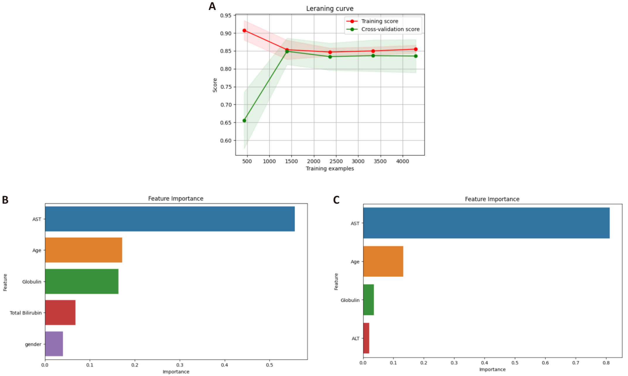
Figure 4. Learning Curves We Plotted. A: Learning curve of our best model (model M11 in Table 3), demonstrating that the model performs well. Feature importance based on (B) RFE and (C) ANOVA feature selection. These are the results of AdaBoost model with ADASYN sampling method which shows the best performance in this study. AST, age, and globulin are the three most important features identified by both feature selection methods.

 

Figures 4B and 4C illustrate the feature importance for models M11 and M12. Both models use the AdaBoost algorithm in combination with ADASYN sampling. The key difference between them is in their feature selection methods: Model M11 uses the RFE technique, while Model M12 employs the ANOVA feature selection approach. The most important features in predicting HPV using the ANOVA feature selection approach are AST, age, globulin, and ALT. These features are well-known indicators of liver function and general health, thus reflecting their importance in modeling HCV. In the case of the RFE method, important features are recognized as AST, age, globulin, total bilirubin, and gender. The inclusion of total bilirubin and gender implies that these features may reveal subtle but meaningful differences in HCV presentation across various demographic groups.

 

The increasing number of desired features may enhance the model's performance, however, it also increases the degree of model complexity which may limit its usage in practice. Hence, limiting the number of the model‘s features to four or five key ones maximizes our model’s practicability by healthcare professionals in early disease detection. The use of limited features in HCV prediction is in agreement with previous studies like Ref.[14] and Ref.[10] in which a limited number of relevant features were employed.

 

6 CONCLUSIONS

Our study demonstrates the importance of choosing the appropriate sampling method to improve the performance of ML models when the dataset is highly imbalanced. The results indicate that the ADASYN sampling method significantly enhances the models' performance. Among the five ML models evaluated, AdaBoost consistently delivered the best performance.

 

The simplicity of our models, requiring only four or five features - depending on the feature selection method employed - to predict HCV infection is a key strength of this study. This eases the use of our models, making it a valuable supplementary tool for doctors in the early diagnosis of disease, which could contribute to saving human lives. For future research, we suggest delving deep into other feature selection and sampling methods and trying different ML models from those used in the current study. Moreover, applying our approach to larger and more diverse datasets from other institutions worldwide could help validate our model's generalizability across different populations. This work could be further extended by introducing additional relevant features to the existing ones which may lead to further improvement in model performance.

 

Acknowledgments

We would like to thank the National Center for Health Statistics (NCHS) for providing us with the datasets used in this study. We also thank the three anonymous reviewers for their constructive comments and valuable suggestions, which have significantly enhanced the quality of our paper. We acknowledge the use of Python and its libraries, including NumPy, pandas, scikit-learn, and Matplotlib for data analysis, ML modeling, and visualizations.

 

Conflicts of Interest

The authors declare no conflicts of interest relevant to this study.

 

Author Contribution

Abbasi M designed the study, conducted part of the ML models, and analyzed the results. Baes M, Abbasi A and Hassanbabaei M conducted part of the ML models and analyzed the results. All authors discussed the results, problems, and methods, interpreted the data, and wrote the paper.

 

Abbreviation List

AC, Acute cholangitis hepatitis

ADASYN, Adaptive Synthetic Sampling

AH, Alcohol-associated hepatitis

ALP, Alkaline phosphates

ALT, Alanine transaminase

ANOVA, Analysis of Variance

AST, Aspartate amino-transferase

AUC, Area under the curve

BMI, Body mass index

EDA, Exploratory Data Analysis

GGT, Gamma-glutamyl transferase

HBV, Hepatitis B virus

HCV, Hepatitis C virus

HHS, United States Department of Health and Human Services 

LASSO, Least Absolute Shrinkage and Selection Operator

ML, Machine learning

NHANES, National Health And Nutrition Examination Survey

NCHS, National Center for Health Statistics

RFE, Recursive feature elimination

SMOTE, Synthetic Minority Over-sampling Technique

SVM, Support vector machine

SVMSMOTE, Support vector machine synthetic minority over-sampling technique

 

References

[1] Tang TQ, Jan R, Shah Z et al. A fractional perspective on the transmission dynamics of a parasitic infection, considering the impact of both strong and weak immunity. PLoS One, 2014; 19: e0297967.[DOI]

[2] Jan R, Hincal E, Hosseini K et al. Fractional view analysis of the impact of vaccination on the dynamics of a viral infection. Alex Eng J, 2024; 102: 36-34.[DOI]

[3] Jan R, Boulaaras S, Alngga M et al. Fractional-calculus analysis of the dynamics of typhoid fever with the effect of vaccination and carriers. Int J Numer Model El, 2023; 37: e3184.[DOI]

[4] Naik PA, Yavuz M, Qureshi S et al. Memory impacts in hepatitis C: A global analysis of a fractional-order model with an effective treatment. Comput Meth Prog Bio, 2024; 254: 108306.[DOI]

[5] Saad KM, Alqhtani M, Gómez-Aguilar JF. Fractal-fractional study of the hepatitis C virus infection model. Results Phys, 2020; 19: 103555.[DOI]

[6] Sadki M, Danane J, Allali K. Hepatitis C virus fractional-order model: mathematical analysis. Model Earth Syst Env, 2023; 9: 1695-1707.[DOI]

[7] Zdrodowska M, Kasperczuk A, Dardzińska-Głębocka A. Selected feature selection methods for classifying patients with Hepatitis C. Procedia Comput Sci, 2023; 225: 3710-3717.[DOI]

[8] Minami T, Masaya S, Hidenori T et al. Machine learning for individualized prediction of hepatocellular carcinoma development after the eradication of hepatitis C virus with antivirals. J Hepatol, 2023; 79: 1006-1014.[DOI]

[9] Ali S, Naveed A, Hussain I et al. Diagnosis and monitoring of hepatocellular carcinoma in Hepatitis C virus patients using attenuated total reflection Fourier transform infrared spectroscopy. Photodiagn Photodyn, 2023; 43: 103677.[DOI]

[10] Ahn JC, Noh YK, Rattan P et al. Machine Learning Techniques Differentiate Alcohol-Associated Hepatitis From Acute Cholangitis in Patients With Systemic Inflammation and Elevated Liver Enzymes. Mayo Clin Proc, 2022; 97: 1326-1336.[DOI]

[11] Park H, Lo-Ciganic W, Huang J et al. Machine Learning Algorithms for Predicting Direct-Acting Antiviral Treatment Failure in Chronic Hepatitis C: An HCV-TARGET Analysis. Hepatology, 2022; 76: 483-491.[DOI]

[12] Farghaly HM, Shams MY, Abd El - Hafeez T. Hepatitis C Virus prediction based on machine learning framework: a real-world case study in Egypt. Knowl Inf Syst, 2023; 65: 2595-2617.[DOI]

[13] Kim SH, Park SJ, Lee H. Machine learning for predicting hepatitis B or C virus infection in diabetic patients. Sci Rep-Uk, 2023; 23: 21518.[DOI]

[14] Lilhore UK, Manoharan P, Simaiya S et al. Hybrid model for precise hepatitis-C classification using improvedrandom forestand SVM method. Sci Rep-Uk, 2023; 13: 12473.[DOI]

[15] Chawla NV, Bowyer KW, Hall LO et al. SMOTE: Synthetic Minority Over-sampling Technique. J Artif Intell Res, 2002; 16: 321-357.[DOI]

[16] He H, Edwardo AG. Learning from imbalanced data. IEEE T Knowl Data Eng, 2009; 21: 1263-1284.[DOI]

[17] Han H, Wang WY, Mao BH. Borderline-SMOTE: A New Over-Sampling Method in Imbalanced Data Sets Learning. In Advances in Intelligent Computing, Springer Berlin Heidelberg, 2005; 878-887.[DOI]

[18] Nguyen HM, Cooper EW, Kamei K. Borderline over-sampling for imbalanced data classification. Int J Knowl Eng Soft Data, 2011; 3: 4-21.[DOI]

[19] He H, Bai Y, Garcia EA et al. ADASYN: Adaptive Synthetic Sampling Approach for Imbalanced Learning. EEE world congress on computational intelligence, IEEE, 2008; 1322-1328. [DOI]

[20] Hosmer Jr DW, Lemeshow S, Sturdivant RX. Applied logistic regression. John Wiley and Sons Press: England, UK, 2013.

[21] Breiman L, Friedman JH, Olshen RA et al. Classification and Regression Trees. CRC press, 1984; 40: 385.[DOI]

[22] Breiman L. Random forests. Mach Learn, 2001; 45: 5-32.[DOI]

[23] Freund Y, Schapire RE. A decision-theoretic generalization of on-line learning and an application to boosting. J Comput Syst Sci, 1997; 55: 119-139.[DOI]

[24] Chen T, Guestrin C. XGBoost: A Scalable Tree Boosting System: Proceedings of the 22nd ACM SIGKDD international conference on knowledge discovery and data mining. San Francisco, USA, 13-17 August 2016.[DOI]

[25] Guyon I, Elisseeff A. An introduction to variable and feature selection. J Mach Learn Res, 2003; 3: 1157-1182.

[26] Hall MA. Correlation-based feature selection for machine learning [PhD Thesis]. Hamilton, IA: University of Waikato; 1999.

[27] Guyon I, Weston J, Barnhill S et al. Gene Selection for Cancer Classification using Support Vector Machines. Mach Learn, 2002; 46: 389-422.[DOI]

[28] Mao Y, PI D, Liu Y et al. Accelerated recursive feature elimination based on support vector machine for key variable identification. Chinese J Chem Eng, 2006; 14: 65-72.[DOI]

[29] Johnson KJ, Synovec RE. Pattern recognition of jet fuels: comprehensive GC× GC with ANOVA-based feature selection and principal component analysis. Chemometr Intell Lab, 2002; 60: 225-237.[DOI]

[30] Kohavi R. A study of cross-validation and bootstrap for accuracy estimation and model selection. LJCAI, 1995; 14: 1137-11145.

[31] Bergstra J, Bengio Y. Random search for hyper-parameter optimization. J Mach Learn Res, 2012; 13.

 

Copyright © 2024 The Author(s). This open-access article is licensed under a Creative Commons Attribution 4.0 International License (https://creativecommons.org/licenses/by/4.0), which permits unrestricted use, sharing, adaptation, distribution, and reproduction in any medium, provided the original work is properly cited.