Mathematical Modeling of Culling and Vaccination for Dog Rabies Disease Transmission with Optimal Control and Sensitivity Analysis Approach

 

Abdulrahman Mumbu1,2*, James David2, Dickson Bahaye2, Jufren Ndendya2,3

 

1Department of Mathematics, Muslim University of Morogoro, Morogoro, Tanzania

2Department of Mathematics, University of Dar es Salaam, Dar es Salaam, Tanzania

3Department of Environmental Health and Ecological Sciences, Ifakara Health Institute, Dar es Salaam, Tanzania

 

*Correspondence to: Abdulrahman Mumbu, PhD, Lecturer and Research Scientist, Department of Mathematics, Muslim University of Morogoro, Morogoro, 53000, Tanzania; Email: amumbu@gmail.com

 

DOI: 10.53964/cme.2025002

 

Abstract

Objective: In this work, a five-compartment mathematical model is developed to investigate the transmission dynamics of rabies infection in dog populations, incorporating vaccination and culling as control interventions. The study also includes an optimal control analysis and a cost-effectiveness evaluation of the proposed interventions.

 

Methods: Local and global stability analyses of the disease-free equilibrium (E₀) and the endemic equilibrium (E*) are established through Jacobian and Lyapunov function techniques, alongside the calculation of the effective reproductive number (Re). A sensitivity analysis is conducted by normalized forward index method to identify key parameters influencing Re. Optimal control and cost-effectiveness techniques were employed to find the optimal and suitable control strategies for the disease control.

 

Results: The study findings indicate that, vaccination rate η1 and force of infection β are the most influential parameters negatively and positively for reducing and increasing Re by -0.8197 and +1.0000 respectively. Also, the work identifies that, combined strategy of vaccination and culling is the most effective approach for controlling rabies within short time, just within 3y, while implementation by using single intervention takes control profile of 4.5y to eliminate the disease. Moreover, the cost-effectiveness analysis shows that, control strategy B is more economically best choice with less incremental cost-effectiveness ratio (ICER) compared to strategies A and C.

 

Conclusion: Therefore, it is recommended that vaccination and culling be implemented simultaneously to significantly reduce the population of exposed and infected dogs, leading to better control of rabies transmission.

 

Keywords: dog rabies, effective reproductive number, vaccination, culling, optimal control

 

1 INTRODUCTION

The Lyssavirus-based disease Rabhas, which means violence in Sanskrit, is a zoonotic carnivore disease that has been known about since 3,000 BC. It has been known for a very long time-more than 4,300 years-and is steadily expanding over numerous nations and locations[1]. An estimated 59,000 people die from the rabies virus each year worldwide[2-4], with roughly 36.4% of those deaths taking place in Africa and 60% in Asia[5,6]. According to WHO[7], this disease causes over 21,000 human deaths per year in the African continent. In 1912, the first cases in the East African region were found in Kenya's Machakos District[8].

 

Even though the disease has been combated with several measures, its annual death toll in the region is still rising, from 210 to 290 for the human population and 4,400 to 6,500 for dogs. In addition to dogs, rabies can infect cats, foxes, skunks, raccoons, and other mammals that carry the virus. Even among different species, dogs continue to be the principal source of rabies disease transmission to humans. When a rabid or sick dog bites another animal or dog, their broken skin, wounds, or scratches get contaminated with virus-laden saliva, which then spreads the disease[9].

 

In the study of Addo[10], the rabies virus enters the spinal cord by the motor pathway, where it becomes infected and quickly spreads to the central nervous system. As soon as the viruses spread to the brain, many behavioral abnormalities started to occur as a result of neuronal defection. The loss of the neurological system causes brain inflammation in the organism, which ultimately leads to death. One way to stop the spread of dog rabies is through vaccination and treatment. Rabies vaccinations for canine or canine populations are administered to susceptible population groups by injection or oral route. By doing this, susceptible dogs who are more prone to contract the disease when socializing with infected dogs will be better protected.

 

Theoretically and experimentally, vaccination is deemed to be successful when it is administered to roughly 70% of the dog population. On the other side, when a dog or canine bites the suspect rabid dog before the infectious stage has formed, a treated population group is enforced[11]. This protects all attacked dogs who have not yet displayed indications of disease infection, but as symptoms emerged, infected dogs stopped receiving treatment and eventually perished. All wounds or scratches should be cleaned and washed completely right away with soap and a clean enough amount of water for around 15mins while also providing supportive care to a victim in any event of a dog bite or any suspected rabid animal[12].

 

The rabies virus continues to be a problem in many places, causing both animal and human deaths, a decline in production due to mortality or incapacity, and the expense of vaccination and treatment operations. More efforts are required to reduce disease spread and fatalities because the disease continues to be prevalent in animal and human populations, particularly in young age groups[13]. The development of effective disease control strategies and a better understanding of the dynamics of infectious disease transmission in a community have both benefited from the use of mathematical models[14]. The several works about the disease infection with various intervention techniques are listed below.

 

In the Bongo District of Ghana, Addo investigated the Susceptible, S(t)Exposed, E(t)-Infected, I(t) and Recovered, R(t) model for rabies transmission infection in the dog population group considering vaccination control intervention. Based on the results, the minimal population coverage of dogs that needed to be immunized was 24.6%. Corresponding to this, the basic reproduction number, R0, with vaccination found as 0.3755 and suggests R0<1, whereas without vaccination intervention it is 1.3267 and implies R0 >1, thus indicating endemic disease status. Similar models were provided by Tulu[15] with the addition of Susceptible, S(t)-Exposed Prodromal, E(t) Infectious, I1(t)-Furious Infectious, I2(t)-Recovery, R(t), which involved the importation of diseased immigrants with the purpose of preventing the spread of the disease among the dog population.

 

In a confined dog population group found in the Machakos District of Kenya, Kital et al.[16] established a model with five classes namely; Susceptible, S(t) Vaccination, V(t)-Latent, L(t)-Infectious, I(t) (SVLI) to investigate the transmission of dog rabies disease with vaccine control techniques. In addition to the analysis of sensitivities, immunization was seen as the best way to stop the spread of disease among dogs. Once more, Carroll et al.[17], and Laager[18] developed a Susceptible, S(t)-Vaccination, V(t)-Exposed, E(t)-Infectious, I(t) model classes in the spreading dynamics of rabies between dog populations by employing immune-contraception method to reduce the number of dogs in cities and towns by means of vaccination alongside dog birth rates control or surgical sterilizing that decreases newborn puppies.

 

Additionally, the model with classes Susceptible, S(t)-Vaccination, V(t)-Exposed, E(t)-Infectious, I(t) was proposed by Fitzpatrick et al.[19] and Bilinski et al.[20], incorporating with a vaccination strategy for rabies disease infection spread control where cost-effectiveness was analyzed for Carnivorous vaccination aim for stopping rabies increase among Ngorongoro and Serengeti districts in Tanzania through controlling dog along with other wildlife community groups. A similar model was also created by Ndii et al.[21] combining crisp and fuzzy techniques, with the primary aspects of transmission beingthe availability of vaccinations and the rate at which infections spread. Leung and Davis[22] suggested a similar mathematical model for administering rabies immunization to the population of owned, free-roaming, and stray dogs.

 

The Susceptible, S(t)-Exposed, E(t)-Infectious, I(t)-Recovered, R(t) model was created and examined by Asamoah et al.[23] and Wiraningsih et al.[24], while Yang and Lou[25] constructed the Susceptible, S(t)-Vaccination, V(t)-Exposed, E(t)-Infectious, I(t) model compartments for the dynamics of rabies disease transmission between dog-human interaction groups with vaccine control measures. In addition, Huang et al.[26] established a comparable model for rabies disease transmission patterns interacting dogs, humans, and Chinese ferret badger communities found in China Zhenjiang Region, while Ega et al.[27] provided a similar work composed of three population groups namely; dogs, human and livestock for analyzing rabies infection transmission employing vaccination control measure in Ethiopia, particularly in Addis Ababa city. In addition, Tian et al.[28] created the model to investigate the trends of the re-emergence of rabies illness spreading in domesticated dogs in Yunnan town, China, and their study used a vaccination control technique incorporating environmental variables to construct a Susceptible, S(t)-Vaccinated, V(t)-Exposed, E(t)-Infectious, I(t) model composed of dog and human interacting groups. Furthermore, Zinsstag et al.[29] built the Susceptible, S(t)-Vaccination, V(t)-Exposed, E(t)-Infectious, I(t) mathematical model with vaccination based on the dog population, purposefully for the spread control of rabies illness between the dog-to-human contacting populations in N'Djamena town, Chad. As others did, their study considered vaccination as a useful approach to illness prevention.

 

In recent times, fractional calculus has gained considerable attention for its application in the study of infectious disease dynamics. Fractional-order models offer a more accurate representation of biological systems by incorporating memory effects, which allow for more realistic descriptions of the spread and control of diseases. These models have been successfully applied to investigate the dynamics of various diseases, including HIV and its interaction with the immune system using non-integer derivatives[30], as well as the dynamics of coronavirus infections under preventive interventions through fractional-calculus analysis[31]. Similarly, the study of plant infections and the implementation of preventive policies have benefited from the dynamical analysis offered by fractional calculus[32].

 

In the context of vector-borne diseases, fractional models have provided valuable insights into the transmission dynamics of dengue, accounting for memory, re-infection, and vaccination[33]. Moreover, chikungunya infection has been studied through fractional calculus, with a focus on evaluating the effects of saturated incidence functions[34]. These studies underscore the significance of fractional-order models in capturing the complexities of infectious disease dynamics more effectively than classical models.

 

Indeed, the current study developed and analyzed a mathematical model of the dog population with classes namely SVEIR (Susceptible, S(t); Vaccinated, V(t); Exposed, E(t); Infectious, I(t); and Recovery, R(t)), for investigating the most influential and potential parameters for dog rabies disease infection spread among the dogs by considering dog vaccination and culling interventions. Additionally, the work made more mathematical applications for its disease optimal control and cost-effectiveness evaluation part for the best use options among the interventions suggested. This aims to control the transmission of disease infection among dogs at minimal cost but with great achievement. Hence, since most of the studies surveyed above missed this angle, this work played a necessary highlight in disease control by considering appropriate and relevant budget use options to attain the planned target.

 

2 MODEL FORMULATION

The model presented here incorporates vaccination for both susceptible and exposed dogs, as well as culling for both exposed and infected dogs as control measures. This model is structured into five compartments, including S(t), V(t), E(t), I(t), and R(t).

 

Following this, the total population is then given by N(t)=S(t)+V(t)+E(t)+I(t)+R(t). Dogs are recruited into the susceptible population group S(t) at the rate of ω. The dog rabies disease infection among the dogs occurs at the rate of β. Vaccination is administered to the susceptible S(t) and exposed E(t) dog groups at the rate of η1 and τ2 respectively, for which some will gain temporary immunity and therefore join to recovered group R(t) through the rate of τ1. Each dog group diminishes due to the natural mortality rate, ϕ2, while the infected dogs I(t) also die due to rabies at the rate of ϕ1. The exposed dog class E(t) develops infection and enters into the infected group I(t) through the rate η2. In both, exposed E(t) and infected I(t) groups, culling c1 and c2 interventions are introduced to control dogs’ reproduction rates growth respectively. The recovered dog group R(t) joins into the susceptible S(t) dogs at the rate of τ3 subject to immune loss. Through these variables and parameters, the following schematic diagram with a set of non-linear ordinary differential equations is established.

 

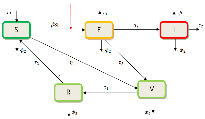
Figure 1. Dog Rabies Disease Schematic Model Diagram.

 

$$ \left\{\begin{array}{c}\frac{{d}{S}}{{d}{t}}=\omega +{{\tau }}_{3}R-\beta SI-\left({{{\eta }}_{1}+{\varphi }}_{2}\right)S\\ \frac{{d}{V}}{{d}{t}}={{\eta }}_{1}S+{{\tau }}_{2}E-\left({{{\tau }}_{1}+{\varphi }}_{2}\right)V\\ \frac{{d}{E}}{{d}{t}}=\beta SI-({{{{\eta }}_{2}+{\tau }}_{2}+{\varphi }}_{2}+{{c}}_{1})E\\ \frac{{d}{I}}{{d}{t}}={{\eta }}_{2}E-({{{\varphi }}_{1}+{\varphi }}_{2}+{{c}}_{2})I\\ \frac{{d}{R}}{{d}{t}}={{\tau }}_{1}V-({{\varphi }}_{2}+{{\tau }}_{3})R\end{array}\right.\left(1\right)$$

 

With the initial conditions; S(0)≥0, V(0)≥0, E(0)≥0, I(0)≥0, R(0)≥0.

 

2.1 Model Analysis

In this section, a region in which solutions of the model system (1) are uniformly bounded in the proper subset Ω∈R5.

 

The total population at any time t is given by

 

N(t)=S(t)+V(t)+E(t)+I(t)+R(t) and

$$ \frac{dN}{dt}=\frac{dS}{dt}+\frac{dV}{dt}+\frac{dE}{dt}+\frac{dI}{dt}+\frac{dR}{dt}\left(2\right)$$

 

Substituting Equation (1) into Equation (2) simplified to

$$ \frac{dN}{dt}=\omega -{\varphi }_{2}N+{c}_{1}E-\left({\varphi }_{1}+{c}_{2}\right)I, \left(3\right)$$

 

In the absence of culling and mortality due to rabies, it becomes

$$ \frac{dN}{dt}\le \omega -{\varphi }_{2}N\left(4\right)$$

 

By solving Equation (4), we obtain 0≤N(t)≤ω/ϕ2.

 

Therefore, the feasible solutions set of the system (1) of the model remain in the region such that:

$$ \Omega =\left\{\left(S\right(t),V(t),E(t),I(t),R(t\left)\right)\in {\mathbb{ℝ}}_{+}^{5}:(S+V+E+I+R)\le \frac{\omega }{{\varphi }_{2}}\right\}$$

 

2.2 Non-Existence of Rabies Disease Equilibrium Point, and Effective Reproduction Number Re

The model system (1) has a disease-free equilibrium point (DFE) obtained by setting the right-hand sides of the equation in the model to zero given by E0=(S0, V0, E0, I0, R0), such that

$$ {E}_{0}=\left[\frac{\omega }{{\varphi }_{2}+{\eta }_{1}},\frac{{\omega \eta }_{1}}{{\varphi }_{2}+{\eta }_{1}},{0,0},0\right]\left(5\right)$$

 

The effective reproduction number of the model system (1), Re is calculated using the Next Generation Matrix method as

$$ {R}_{e}=\frac{\beta \omega {\eta }_{2}}{({{{\eta }_{2}+\tau }_{2}+\varphi }_{2}+{c}_{1})({{\varphi }_{2}+\varphi }_{1}+{c}_{2})({\varphi }_{2}+{\eta }_{1})}\left(6\right)$$

 

2.3 Rabies Disease Existence Equilibrium Point

The endemic equilibrium pointE1 and defined as a steady state for the model system (1). This occurs when there is a persistence of the disease. It can be obtained by equating the system of Equation (1) to zero. Then we obtain

 

$$ {E\ast =[S}^{\ast },{V}^{\ast },{E}^{\ast }, {I}^{\ast },{R}^{\ast }\left]\right(7)$$

 

such that:

$$ {S}^{*}=\frac{({{{\eta }_{2}+\tau }_{2}+\varphi }_{2}+{c}_{1})({{\varphi }_{2}+\varphi }_{1}+{c}_{2})}{\beta {\eta }_{2}}$$

$$ {V}^{*}=\frac{{{\eta }_{1}{S}^{*}+\tau }_{2}{E}^{*}}{{\varphi }_{2}+{\tau }_{1}}$$

$$ {E}^{*}=\frac{({{\varphi }_{2}+\varphi }_{1}+{c}_{2})}{{\eta }_{2}}\times {I}^{*}$$

$$ {I}^{*}=\frac{({{{\eta }_{2}+\tau }_{2}+\varphi }_{2}+{c}_{1})}{{\beta S}^{*}}\times {E}^{*}$$

$$ {R}^{*}=\frac{{\tau }_{1}{V}^{*}}{{{\tau }_{3}+\varphi }_{2}}$$

 

2.4 Local Stability of Non-existence of Dog Rabies Disease Steady State E0

We linearize the system in (1) to obtain the Jacobian Matrix J(E0) at E0 to determine the local stability of DFE dog rabies as;

$$ {J}\left({E}_{0}\right)=\left(\genfrac{}{}{0pt}{}{\begin{array}{c}-\left({{\varphi }}_{2}+{{\eta }}_{1}\right)\\ {{\eta }}_{1}\end{array}}{\begin{array}{c}0\\ 0\\ 0\end{array}}\genfrac{}{}{0pt}{}{\begin{array}{c}0\\ -\left({{\varphi }}_{2}+{{\tau }}_{1}\right)\end{array}}{\begin{array}{c}0\\ 0\\ {{\tau }}_{1}\end{array}}\genfrac{}{}{0pt}{}{\begin{array}{c}0\\ {{\tau }}_{2}\end{array}}{\begin{array}{c}-\left({{\varphi }}_{2}+{{\eta }}_{2}+{{\tau }}_{2}+{{c}}_{1}\right)\\ {{\eta }}_{2}\\ 0\end{array}}\genfrac{}{}{0pt}{}{\begin{array}{c}-\beta S\\ 0\end{array}}{\begin{array}{c}\beta S\\ -\left({{\varphi }}_{2}+{{\varphi }}_{1}+{{c}}_{2}\right)\\ 0\end{array}}\genfrac{}{}{0pt}{}{\begin{array}{c}{{\tau }}_{3}\\ 0\end{array}}{\begin{array}{c}0\\ 0\\ -\left({{\varphi }}_{2}+{{\tau }}_{3}\right)\end{array}}\right)\left(8\right)$$

 

From Equation (8), trace-determinant approach is applied to determine local stability analysis[35], in which for trace TrJ(E0) we get TrJ(E0) = -5ϕ2-τ1-η1-c1-η2-τ2-c2-ϕ1-τ3;

$$ \therefore TrJ\left({E}_{0}\right)<0.\left(9\right)$$

 

Consequently, the determinant Det J(E0) is obtained as

$$ DetJ\left({E}_{0}\right)=\left(\beta \omega \eta 2\left(\varphi 2+\tau 1\right)\left(\varphi 2+\tau 3\right)-{k}_{2}\right)-\left(\beta \omega \eta 2\left(\varphi 2+\tau 1\right)\left(\varphi 2+\tau 3\right)\right)$$$$ -{k}_{1}(\varphi 2+\eta 2+\tau 2+c1)(\varphi 2+\varphi 1+c2-k2)\left(10\right)$$

 

Through several simplifications and substitutions, obvious Det J(E0)>0, if the following achieved

 

$$DetJ\left({E}_{0}\right)={k}_{1}\left(\varphi 2+\eta 2+\tau 2+c1\right)\left(\varphi 2+\varphi 1 +c2\right)+2{k}_{2}\left[1-Re\right]\left(11\right)$$

 

By using the condition in Equation (11) clearly, Det J(E0)>0 for Re<1, which implies that, biologically, rabies disease infection will be easily exited from the particular population, and this establishes the following theorem:

Theorem 1. The DFE point of the model (1), given by E0, is locally asymptotically stable (LAS) if Re<1 and unstable if Re >1.

 

2.5 Global Stability Analysis of Non-existence of Dog Rabies Disease Equilibrium Point

To compute the global stability of E0, we choose and employ the Lyapunov function L technique below[36]

$$ L=\left(S-{S}_{0}-{S}_{0}In\frac{S}{{S}_{0}}\right)+\left(V-{V}_{0}-{V}_{0}In\frac{V}{{V}_{0}}\right)+{r}_{1}E+{r}_{2}I+\left(R-{R}_{0}-{R}_{0}In\frac{R}{{R}_{0}}\right) \left(12\right)$$

 

Taking derivatives in Equation (12) with respect to time t we obtain;

$$ \frac{dL}{dt}=\left(1-\frac{S}{{S}_{0}}\right)\frac{dS}{dt}+\left(1-\frac{V}{{V}_{0}}\right)\frac{dV}{dt}+{r}_{1}\frac{dE}{dt}+{r}_{2}\frac{dI}{dt}+\left(1-\frac{R}{{R}_{0}}\right)\frac{dR}{dt}\left(13\right)$$

 

Using substitutions, Equation (13) becomes:

 

$$ \frac{dL}{dt}=\left(1-\frac{S}{{S}_{0}}\right)\left[\omega +{\tau }_{3}R-\beta SI-\left({{\eta }_{1}+\varphi }_{2}\right)S\right]$$

$$ +\left(1-\frac{V}{{V}_{0}}\right)\left[{\eta }_{1}S+{\tau }_{2}E-\left({{\tau }_{1}+\varphi }_{2}\right)V\right]+{r}_{1}\left[\beta SI-\left({{{\eta }_{2}+\tau }_{2}+\varphi }_{2}+{c}_{1}\right)E\right]$$

$$ +{r}_{2}\left[{\eta }_{2}E-\left({{\varphi }_{1}+\varphi }_{2}+{c}_{2}\right)I\right]+\left(1-\frac{R}{{R}_{0}}\right)\left[{\tau }_{1}V-\left({\varphi }_{2}+{\tau }_{3}\right)R\right] \left(14\right)$$

 

Explicitly, assume that; S≤S0, V≤V0, and R≤R0, consequently Equation (15) is obtained through substitution and simplifications in Equation (14).

$$ \frac{dL}{dt}\le {{r}}_{1}\left({{R}}_{{e}}-1\right)\left(15\right)$$

 

Therefore, by considering positive constants r1 and r2 in the trivial equilibrium points E0, it is obvious that Equation (15) derives the following theorem:

Theorem 2. If Re≤1, then the disease-free equilibrium point E0 is globally asymptotically stable, while for Re>1 will be unstable in the region Ω.

 

2.5.1 Global Stability for the Disease Existence Equilibrium

To determine the global stability of rabies disease existence endemic equilibrium E∗, appropriate Lyapunov function W technique is selected and is defined as:

$$ W\left({x}_{1},...,{x}_{n}\right)=\sum _{i=1}^{5}\frac{1}{2}{\left[{x}_{i}-{x}_{i}^{\ast }\right]}^{2}\left(16\right)$$

 

where xi presents all dog population compartments and implies dog classes dominated with rabies disease infection at E∗.

 

Then Equation (16) can be expressed as

$$ {\begin{array}{c}W\left(S\right(t),V(t),E(t), I(t), R(t\left)\right)=\frac{1}{2}\left[\right(S-{S}^{*})+(V-{V}^{*})\\ +(E-{E}^{*})+(I-{I}^{*})+(R-{R}^{*})]\end{array}}^{2} \left(17\right)$$

 

Taking derivatives with respect to time t in Equation (17) leads to

$$ \frac{dW}{dt}=\left[\left(S-{S}^{\ast }\right)+\left(V-{V}^{\ast }\right)+\left(E-{E}^{\ast }\right)+\left(I-{I}^{\ast }\right)+\left(R-{R}^{\ast }\right)\right]$$$$ \frac{d}{dt}\left[S+V+E+I+R\right]\left(18\right)$$

 

Remember Equation (2), where we get:

$$ \frac{dN\left(t\right)}{dt}=\frac{d}{dt}\left[S+V+E+I+R\right]\left(19\right)$$

 

By employing Equation (2), and using Equation (1) and Equation (19) followed by simplifications gives:

$$ \frac{dN\left(t\right)}{dt}=\omega -{\varphi }_{2}N\left(t\right),\left(20\right)$$

 

Similarly, we have also:

$$ {S}^{\ast }+{V}^{\ast }+{E}^{\ast }+{I}^{\ast }+{R}^{\ast }=\frac{\omega }{{\varphi }_{2}}\left(21\right)$$

 

By combining Equations (20), and (21), then Equation (18) is simplified to:

$$ \frac{dW}{dt}=\left[N\left(t\right)-\frac{\omega }{{\varphi }_{2}}\right]\left[\omega -{\varphi }_{2}N\left(t\right)\right]\left(22\right)$$

 

Consequently, by simplifying and re-arranging in Equation (22), we obtain:

$$ \frac{dW}{dt}=-\frac{1}{{\varphi }_{2}}{\left[\omega -{\varphi }_{2}N\left(t\right)\right]}^{2}<0\left(23\right)$$

 

Hence, Equation (23) concludes the proof of global stability (GS) at E∗ such that dW/dt＜0 a strictly Lyapunov function achieved indicates that, at E∗ dog rabies disease is globally asymptotically stable and is contained in the defined region Ω. This leads to the following theorem:

Theorem 3. If Re>1, then the existing endemic equilibrium point E∗ is globally asymptotically stable (GAS) which is contained in the defined region Ω.

 

2.6. Sensitivity Analysis

Conducting a sensitivity analysis allows us to assess how the model parameters influence the effective reproduction number (Re) and, consequently, disease transmission[37]. This analysis provides insights into which parameters and initial conditions influence the model’s outcomes and helps pinpoint parameters that warrant further numerical investigation[38].

 

The normalized sensitivity index (SI) of the variable Re depends on the differentiability of a parameter l that is defined as;

$$ {{{\rm Y}}}_{l}^{{R}_{e}}=\frac{\partial {R}_{e}}{\partial l}\times \frac{l}{{R}_{e}},$$

where l is any parameter presented in effective reproduction number Re. For example, the sensitivity index of Re corresponding to the parameter ϕ1 is given as

$$ {{{\rm Y}}}_{l}^{{R}_{e}}=\frac{\partial {R}_{e}}{\partial {\varphi }_{1}}\times \frac{{\varphi }_{1}}{{R}_{e}}=-0.621118$$

 

Other indices are calculated using a similar approach and the results are displayed in Table 1.

 

Table 1. Parameter Values and Sensitivity Indices (SI) of the Model corresponding to Re.

 

From indices in Table 1, we have a SI profile which can be presented in bar graph as shown in Figure 2.

 

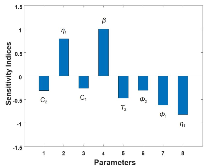
Figure 2. Graph of sensitivity indices of Re with respect to the model parameters.

 

Figure 2 illustrates the SI profile of Re concerning all parameters within the model system (1). A negative value signifies that an augmentation in the parameter value results in a reduction of Re, whereas a positive value denotes that an increase in the parameter value leads to an elevation in Re. Consequently, β exhibits an index value of +1.0000, making it the most positively sensitive parameter, while η1 holds an index value of -0.8197, signifying it as the most negatively sensitive parameter.

 

2.6.1 Interpretation of the sensitivity

The sensitivity analysis of the model’s parameters revealed valuable insights. Parameters β and η2 exhibited positive indices, indicating their significant impact on the model. Notably, β had the highest positive index, suggesting that increasing this parameter would elevate the effective reproduction number Re and, consequently, the risk of a disease outbreak.

 

Conversely, parameters such as c1, c2, τ2, ϕ2, ϕ1, and η1 displayed negative indices, indicating their potential to reduce Re when their values increase. Among these, the Susceptible vaccination rate (η1=-0.819672) was the most influential in decreasing the disease burden among dogs.

 

In summary, the sensitivity analysis underscores the importance of enhancing the efficacy of vaccination by targeting the S class and implementing vaccination for the E class, along with culling for E and I classes, and considering the natural death rate. Additionally, reducing the contact rate between S and I dogs can also effectively curb the spread of Dog rabies. Therefore, it is crucial to maintain and expand vaccination and culling programs as vital strategies to combat the transmission of Dog rabies infection.

 

2.7 Optimal Control Formulation

We apply optimal control techniques to the model system (1) in this section. Our goals are to reduce the number of cases of dog rabies as well as the expenses related to control measures. To stop the spread of dog rabies, we add culling u2 (0≤u2≤1) and vaccination u1(0≤u1≤1) as time-dependent controls to the model system (1). Next, the model system (1) turns into

 

$$ \left\{ \begin{array}{c}\frac{dS}{dt}=\omega +{\tau }_{3}R-\beta SI-(1+{u}_{1}){{\eta }_{1}S-\varphi }_{2}S\\ \frac{dV}{dt}={(1+{u}_{1})\eta }_{1}S+(1+{u}_{1}){\tau }_{2}E-\left({{\tau }_{1}+\varphi }_{2}\right)V\\ \frac{dE}{dt}=\beta SI-(1+{u}_{1}){\tau }_{2}E-{{(\eta }_{2}+\varphi }_{2})E-{(1+{u}_{2})c}_{1}E\\ \frac{dI}{dt}={\eta }_{2}E-\left({{\varphi }_{1}+\varphi }_{2}\right)I-{(1+{u}_{2})c}_{2}I\\ \frac{dR}{dt}={\tau }_{1}V-({\varphi }_{2}+{\tau }_{3})R\end{array}\right.\left(24\right)$$

 

to study the optimal control level of the controls, the control set U, which is Lebesgue measurable is defined as U={(u1, u2): 0≤u1≤1, 0≤u2≤1, 0≤t≤tf}.

 

The purpose of introducing the controls in the model system is to find the optimal level of the intervention strategy to reduce the spread of dog rabies disease and the cost of implementing the controls. The control variables u1 and are minimized subject them to the differential Equation (24), where we formulate the objective function as

$$ {J}_{({u}_{1},{u}_{2})}={\int }_{0}^{tf}{[A}_{1}E+{A}_{2}I+\frac{1}{2}({c}_{1}{u}_{1}^{2}+{c}_{2}{u}_{2}^{2})\left]dt\right(25)$$

where tf is the final time, while A1, A2, c1 and c2 are positive weights. The expression represents the costs associated with the control u1 and u2. The objective function (25) involves minimizing the number of dog rabies infections (E and I) as well as the cost of applying the control strategies u1 and u2. Thus, we seek to find the optimal controls and such that

$$ {J}_{({u}_{1}^{\ast },{u}_{2}^{\ast })}=Min\left\{J\left({u}_{1},{{u}}_{2}\right):{u}_{1},{{u}}_{2}\in U\right\}\left(26\right)$$

where; U={(u1, u2) : 0 ≤ u1 ≤ 1,0 ≤ u2 ≤ 1,0 ≤ t ≤ tf}.

 

By using Potryagin's maximum principle[42], we drive the necessary conditions for our optimal control and corresponding states. This principle converts the system of Equations (25) and (26) into the problem of minimizing point-wise a Hamiltonian (H), with respect to u1(t) and u2(t)

$$ {{H}={A}}_{1}{E}+{{A}}_{2}{I}+\frac{1}{2}{c}_{1}{u}_{1}^{2}+\frac{1}{2}{c}_{2}{u}_{2}^{2}+{\lambda }_{1}\left[\omega +{\tau }_{3}R-\beta SI-\left(1+{u}_{1}\right){{\eta }_{1}S-\varphi }_{2}S\right]$$$$ +{\lambda }_{2}\left[{\left(1+{u}_{1}\right)\eta }_{1}S+\left(1+{u}_{1}\right){\tau }_{2}E-\left({{\tau }_{1}+\varphi }_{2}\right)V\right]$$$$ +{\lambda }_{3}[\beta SI-(1+{u}_{1}){\tau }_{2}E-{{(\eta }_{2}+\varphi }_{2})E-{\left(1+{u}_{2}\right)c}_{1}E]$$$$ +{\lambda }_{4}[{\eta }_{2}E-({{\varphi }_{1}+\varphi }_{2})I-{\left(1+{u}_{2}\right)c}_{2}I]+{\lambda }_{5}[{\tau }_{1}V-({\varphi }_{2}+{\tau }_{3}\left)R\right]\left(27\right)$$

 

where λ1, λ2, λ3..., λ5 are the co-state variables or the adjoint variables associated by S, V, E, I and R. The adjoint equations are obtained by

 

$$ \left\{\begin{array}{c}\frac{d{\lambda }_{1}}{dt}=-\frac{\partial H}{\partial S}={(\lambda }_{1}{-\lambda }_{2}\left)\right(1+{u}_{1}){\eta }_{1}+{(\lambda }_{1}{-\lambda }_{3})\beta I+{\lambda }_{1}{\varphi }_{2}\\ \frac{d{\lambda }_{2}}{dt}=-\frac{\partial H}{\partial V}={{(\lambda }_{2}{-\lambda }_{5})\tau }_{1}+{\lambda }_{2}{\varphi }_{2}\\ \frac{d{\lambda }_{3}}{dt}=-\frac{\partial H}{\partial E}=-{A}_{1}+{\lambda }_{3}\left({{\varphi }_{2}+(1+{u}_{2})c}_{1}\right)+{(\lambda }_{3}{-\lambda }_{4}){\eta }_{2}?\\ +{(\lambda }_{3}{-\lambda }_{2}\left)\right(1+{u}_{1}){\tau }_{2}\\ \frac{d{\lambda }_{4}}{dt}=-\frac{\partial H}{\partial I}=-{A}_{2}+{(\lambda }_{1}{-\lambda }_{3}\left)\beta S?{+\lambda }_{4}\right({\varphi }_{1}+{\varphi }_{2}+{(1+{u}_{2})c}_{2})\\ \frac{d{\lambda }_{5}}{dt}=-\frac{\partial H}{\partial R}={{(\lambda }_{5}{-\lambda }_{1})\tau }_{3}+{\lambda }_{5}{\varphi }_{2}\end{array}\left(28\right)\right.$$

 

with the final time conditions (transversality conditions):

$$ {\lambda }_{1}\left({T}_{f}\right)={\lambda }_{2}\left({T}_{f}\right)={\lambda }_{3}\left({T}_{f}\right)={\lambda }_{4}\left({T}_{f}\right)={\lambda }_{5}\left({T}_{f}\right)={\lambda }_{6}\left({T}_{f}\right)=0\left(29\right)$$

 

Moreover, the control set is characterized by;

$$ \frac{\partial H}{\partial {u}_{i}}=0⟹\frac{\partial H}{\partial {u}_{1}}=\frac{\partial H}{\partial {u}_{2}}=0\left(30\right)$$

then,

$$ \left\{\begin{array}{c}\frac{\partial H}{\partial {u}_{1}}={c}_{1}{u}_{1}+({\lambda }_{2}-{\lambda }_{1}){\eta }_{1}S+({\lambda }_{2}-{\lambda }_{3}){\tau }_{2}E,\\ \frac{\partial H}{\partial {u}_{2}}={c}_{2}{u}_{2}+{\lambda }_{3}{c}_{1}E-{\lambda }_{4}{c}_{2}I\end{array}\right. \left(31\right)$$

 

Solving (31) for and when ∂H/∂ui=0 gives;

$$ \left\{\begin{array}{c}{u}_{1}^{\ast }=\frac{({\lambda }_{1}-{\lambda }_{2}){\eta }_{1}{S}^{\ast }+({\lambda }_{3}-{\lambda }_{2}){\tau }_{2}{E}^{\ast }}{{c}_{1}},\\ {u}_{2}^{\ast }=\frac{{\lambda }_{3}{c}_{1}{E}^{\ast }-{\lambda }_{4}{c}_{2}{I}^{\ast }}{{c}_{2}}\end{array}\right.\left(32\right)$$

 

Therefore,

$$ {u}_{1}^{\ast }=min\left\{1,max\left\{0, \frac{({\lambda }_{1}-{\lambda }_{2}){\eta }_{1}{S}^{\ast }+({\lambda }_{3}-{\lambda }_{2}){\tau }_{2}{E}^{\ast }}{{c}_{1}}\right\}\right\},$$$$ {u}_{2}^{\ast }=min\left\{1, max\left\{0, \frac{{\lambda }_{3}{c}_{1}{E}^{\ast }-{\lambda }_{4}{c}_{2}{I}^{\ast }}{{c}_{2}}\right\}\right\}\left(33\right)$$

 

2.8 Numerical Simulation

In this section, the forward and backward fourth-order Runge-Kutta methods implemented in MATLAB (R2022a) software were used to solve the optimal system results within an interval of [0,5] years. The method was chosen because of its accuracy, versatility, stability, and ease of implementation. Simulation of the model system (1) was done using the parameters in the Table 1, and we use the initial population of dogs as; S=1000, V=600, E=300, I=100, R=200.

 

To ensure, a balanced consideration of terms within the objective function aimed at minimizing infectious impacts, equal weight constants are chosen, resulting in A1=A2=1. Additionally, the weight constants used to gauge the expenses associated with implementing control strategies are specified as C1=10, and C2=10.

 

2.8.1 Control with Vaccination Alone

Figure 3 shows how the single implementation of Vaccination, u1(t), affects the spread of dog rabies dynamics in the population. The results in Figure 3A and B show a significant difference in the number of infected individuals in the Exposed, and infected stages with vaccination control compared to the number without control. Due to control u1, the number of infected dogs decreases from 100 to approaching zero after 3 years duration, while the exposed were declined from nearly 350 to about non-existence during the 2.5th year.

 

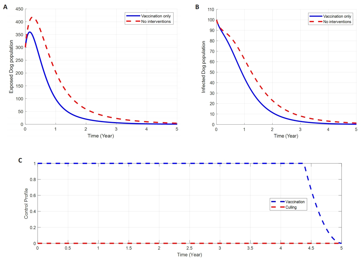
Figure 3. The Impact of Vaccination on Dog Rabies Diseases Dynamics. A: Impacts of vaccination on exposed dogs. B: Impacts of vaccination on infected dogs. C: Profile control of dog rabies disease through vaccination intervention alone.

 

However, vaccination has shown a greater impact on Exposed dogs compared to Infected Dogs. Figure 3C shows the control profile of (u1) in which the control u1 is at the upper bound until the time t=4.5 years, before slowly dropping to the lower bound at the final time.

 

2.8.2 Control with Culling alone

Figure 4 shows how the single implementation of the Culling control strategy, u2(t), affects the transmission dynamics of Dog Rabies disease in a population. The results in Figure 4A-B show a significant difference in the number of infected Dogs in the Exposed and Infected stages with Culling control compared to the number without control. Due to the control u2, the number of exposed ans infected Dogs decreases from 350 and 100 respectively to nearly zero after 2.5th time duration. However, Culling therapy has shown a greater impact on Infected.

 

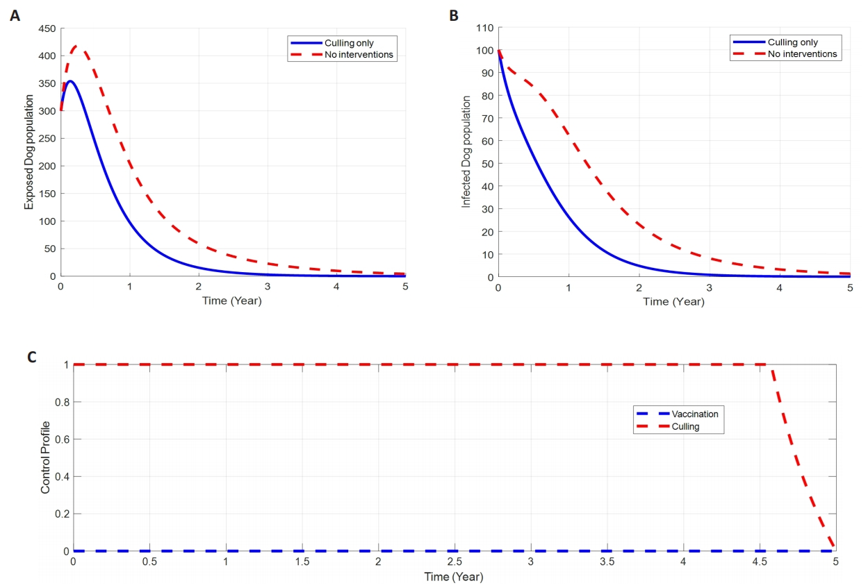
Figure 4. The Impact of Culling on Dog Rabies Diseases Dynamics. A: Impacts of culling on exposed dogs. B: Impacts of culling on infected dogs. C: Profile control of dog rabies disease through culling intervention alone.

 

Dogs’ population compared to Exposed. Figure 4C shows the control profile of (u2) in which the control u2 is at the upper bound until the time t=4.7, before slowly dropping to the lower bound at the final time.

 

2.8.3 Control with Both Interventions (Vaccination and Culling)

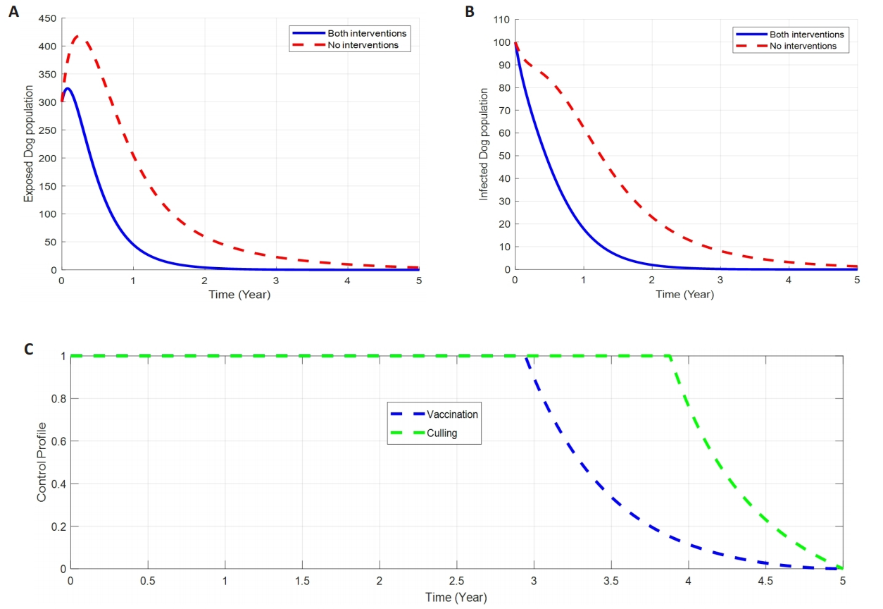
Figure 5. The Impact of Both Interventions (Vaccination And Culling) on Dog Rabies Disease Dynamics. A: Impacts of vaccination and culling on exposed dogs. B: Impacts of vaccination and culling on infected dogs. C: Profile control of dog rabies disease through vaccination and culling intervention.

 

In this strategy, the implementation of both control strategies, Vaccination (u1), and Culling (u2), is used to minimize the objective function in (25). The results in Figure 5A-B demonstrate a significant reduction in the number of exposed and infected Dogs with the existence of combined control strategies compared to when the control strategies are not in place. Figure 5C shows the control profile in which the control strategy (u1) is maintained at a maximum effort of 100% until t=3, (u2) is maintained at the maximum effort of 100% until t=4 for infected individuals in the population, before gradually dropping to the lower bound at the final time. Therefore, it is clear that, employing both strategies brings quicker impacts in reducing the number of exposed and infected dogs compared with the application of single strategy intervention.

 

2.9 Cost-Effectiveness Analysis

In this section, we conduct a cost-effectiveness analysis (CEA) with the aim of identifying the most cost-effective control measure, whether it’s a single strategy or a combination of two, in order to minimize disease infections while optimizing cost-efficiency. To accomplish this, we employ the Incremental Cost-Effectiveness Ratio (ICER). The ICER plays a crucial role in discerning the most economically efficient strategy for mitigating the spread of Dog Rabies disease by comparing any two competing measures. This methodology is particularly valuable when allocating limited resources for disease control, as explained by Olaniyi et al.[43]

 

Change in the total costs of control measures

$$ ICER=\frac{{C}{h}{a}{n}{g}{e}{i}{n}{t}{h}{e}{t}{o}{t}{a}{l}{c}{o}{s}{t}{s}{o}{f}{c}{o}{n}{t}{r}{o}{l}{m}{e}{a}{s}{u}{r}{e}{s}}{{C}{h}{a}{n}{g}{e}{i}{n}{t}{h}{e}{n}{u}{m}{b}{e}{r}{o}{f}{i}{n}{f}{e}{c}{t}{i}{o}{n}{s}{a}{v}{e}{r}{t}{e}{d}}\left(34\right)$$

 

Change in the number of infections averted

 

$$ totalCost\left({C}_{T}\right)={\int }_{0}^{{T}_{f}}({C}_{1}{u}_{1}\left(S\left(t\right)+E\left(t\right)\right)+{C}_{2}{u}_{2}\left(E\left(t\right)+I\left(t\right)\right)dt,(35)$$

 

where C1 and C2 correspond to per dog unit cost based on the use of Vaccination (u1) and per Dog unit cost of Culling (u2) of susceptible, Exposed, and Infected Dogs respectively.

 

Table 2. Number of Infections Averted and Total Cost of Each Strategy

 

The results obtained (as depicted in Table 2) reveal that the ICER value for strategy C surpasses that of strategy A. This implies that implementing all control measures is more expensive and less effective than when solely employing control u1 (Vaccination). Consequently, strategy C is excluded from the roster of viable control strategies.

 

By examining results in Table 2, the competing strategy A with strategy B it becomes evident that the Incremental Cost-Effectiveness Ratio (ICER) for strategy A exceeds the ICER value for strategy B. This signifies that strategy A is decidedly inferior, implying higher costs and lower effectiveness compared to strategy B. As a result, strategy B, which involves culling, emerges as the most economically efficient option among the three strategies.

 

Consequently, the adoption of culling is deemed the optimal and most cost-effective intervention for significantly reducing the prevalence of Dog Rabies disease within the population.

 

3 DISCUSSION

In this study, we developed and analyzed the dog rabies disease model comprises of five compartments of dog population to evaluate the impacts of vaccination and culling intervention approaches for the disease control. Effective reproduction number (Re) was computed by the Next Generation method which is potential key for the disease prevalence. Again, both equilibrium points for disease free and endemic were determined accordingly followed by their respective analyses. Analytically, we observed that at disease free equilibrium point (E0) potentially Re<1 exists, which implies that the dog rabies disease is weak, and consequently easily for its elimination and control. However, for the endemic equilibrium point (E*) we see the reverse that Re>1 persists suggesting that the disease is strong enough to remain in the population at significant time duration. Furthermore, we computed for the sensitivity analysis to identify the most and significant influential parameters that contribute to the existence and elimination of the disease in the population.

 

The study also introduces an optimal control model aimed at evaluating the effectiveness of various strategies for managing rabies transmission in dog populations. The model investigates time-dependent control measures, such as vaccinating both susceptible and exposed dogs, as well as implementing culling strategies to reduce the number of infected animals. To identify the optimal control conditions, Pontryagin’s Maximum Principle is applied, followed by numerical simulations using the forward and backward fourth-order Runge-Kutta methods.

 

Our findings show that, with the implementation of a single control strategy either vaccination (u1) or culling (u2) alone brings a little impact on reducing the dog rabies disease infection as it takes almost 2.5 to 3 years duration to eliminate the number of exposed and infected dogs in the population as seen and discussed in Figure 3 and Figure 4A-B. Moreover, the disease control profile time for single intervention is more prolonged to almost 4.5 years before bringing its impacts on the disease control (refer Figures 3 to 4C).

 

On the other hand, the study suggesting that, the utilization of both interventions simultaneously, that’s vaccination and culling give more significant reduction of exposed and infected number of dogs from its peak of 350 and 100 respectively, to approaching zero for about 1.5y duration (Figure 5A-B). Additionally, double interventions (vaccination and culling) bring a potential impact on the disease control profile time from 4.5 to 3 and 4 years for the vaccination and culling respectively.

 

Furthermore, from the Table 2 above, a cost-effectiveness analysis further identifies culling (strategy B) as the most economically efficient approach, showing the lowest incremental cost-effectiveness ratio -0.01012856 compared with other strategies (A=0.00028675 and C=0.00479694), particularly when implemented on a larger scale. However, this option is convincing economically, but not sufficient in combating infection spread in the dog population timely.

 

These findings align with previous studies on infectious disease control, where fractional-calculus-based models have provided deeper insights into the dynamics of diseases like monkey-pox and HIV[44]. Fractional calculus has proven useful in capturing memory effects and variable transmission factors, as seen in models for diseases such as Hand-Foot-Mouth Disease[45]. Furthermore, the study’s use of optimal control strategies is consistent with approaches seen in modelling water-borne diseases, where non-singular and non-local kernels are employed to reflect the complex nature of disease transmission[46]. The inclusion of fractional derivatives could enhance future rabies models by accounting for long-term effects and delayed responses, as demonstrated in the analysis of HIV transmission dynamics via the Galerkin method[47].

 

4 CONCLUSION

Ultimately, this study suggests that effective rabies control can be achieved by simultaneously implementing vaccination and culling, particularly targeting the exposed and infectious dog populations, which plays a critical role in sustaining the disease, although on the economical basis does not give optimal solution for combination of control strategy  alternatives obtained.

 

Acknowledgements

This work has been supported by the Mathematics for Sustainable Development (MATH4SDG) project, which is a research and development project running in the period 2021-2026 at Makerere University-Uganda, University of Dar es Salaam -Tanzania, and the University of Bergen-Norway, funded through the NORHED II program under the Norwegian Agency for Development Cooperation (NORAD, project No. 68105).

 

Conflicts of Interest

The authors declared no conflict of interest.

 

Data Availability

All supportive data regarding this work are included.

 

Copyright and Permissions

Copyright © 2025 The Author(s). Published by Innovation Forever Publishing Group Limited. This open-access article is licensed under a Creative Commons Attribution 4.0 International License (https://creativecommons.org/licenses/by/4.0), which permits unrestricted use, sharing, adaptation, distribution, and reproduction in any medium, provided the original work is properly cited.

 

References

[1] Takayama N. Rabies: A preventable but incurable disease. J Infect Chemother, 2008; 14, 8-14.[DOI]

[2] Hampson K, Coudeville L, Lembo T et al.  Estimating the global burden of endemic canine rabies. Plos Neglect Trop D, 2015; 9.e0003709.[DOI]

[3] Czupryna AM, Brown JS, Bigambo MA et al.  Ecology and Demography of Free-Roaming Domestic Dogs in Rural Villages near Serengeti National Park in Tanzania. PLoS One, 2016; 11: e0167092.[DOI]

[4] Sambo M, Johnson PC, Hotopp K et al. Comparing Methods of Assessing Dog Rabies Vaccination Coverage in Rural and Urban Communities in Tanzania. Front Vet Sci, 2017; 4: 33.[DOI]

[5] Mpolya EA, Lembo T, Lushasi K et al. Toward Elimination of Dog-Mediated Human Rabies: Experiences from Implementing a Large-scale Demonstration Project in Southern Tanzania. Front Vet Sci, 2017; 4: 21.[DOI]

[6] Pieracci EG, Scott TP, Coetzer A et al.  The Formation of the Eastern Africa Rabies Network: A Sub-Regional Approach to Rabies Elimination. Trop Med Infect Dis, 2017; 2: 29.[DOI]

[7] World Health Organization WHO (2018) Expert Consultation on Rabies, third report. Geneva: (WHO Technical Report Series, No. 1012). Licence: CC BY-NCSA 3.0 IGO.

[8] Borus P. Rabies: the emergence of a microbial threat. E Afr Med J, 1996; 73, 32-34.

[9] Borse RH, Atkins CY, Gambhir M et al. Cost-effectiveness of dog rabies vaccination programs in East Africa. Plos Neglect Trop Ds, 2018; 12: e0006490.[DOI]

[10] Addo, KM. An SEIR Mathematical Model for Dog Rabies. Case Study: Bongo District, Ghana. MSc. Dissertation Kwame Nkrumah University of Science and Technology, 2012.

[11] Guo C, Li Y, Huai Y, Rao CY et al. Exposure history, postexposure prophylaxis use, and clinical characteristics of human rabies cases in China 2006-2012. Sci Rep, 2018; 8: 17188.[DOI]

[12] Ward JKR, Smith GC, Massei G. Disease transmission mode has little effect on simulated canine rabies elimination. CC-BY 4.0 International license. 2018.[DOI]

[13] Kipanyula MJ. Why has canine rabies remained endemic in the Kilosa district of Tanzania? Lessons learnt and the way forward. Infect Dis Poverty, 2015; 4: 1-7.[DOI]

[14] Naveed M, Baleanu D, Raza A et al. Modelling the transmission dynamics of delayed pneumonia-like diseases with a sensitivity of parameters. Adv Differ Equ-Ny, 2021; 2021: 1-19.[DOI]

[15] Tulu AM, Koya PR. The Impact of Infective Immigrants on the Spread of Dog Rabies. Am J Appl Math, 2017; 5, 68-77.[DOI]

[16] Kitala PM, McDermott JJ, Coleman PG et al. Comparison of vaccination strategies for the control of dog rabies in Machakos District, Kenya. Epidemiol Infect, 2002; 129: 215-222.[DOI]

[17] Carroll MJ, Singer A, Smith GC et al. The use of immuno-contraception to improve rabies eradication in urban dog populations. Wildlife Res, 2010; 37: 676-687.[DOI]

[18] Laager M, Lechenne M, Naissengar K et al. A metapopulation model of dog rabies transmission in N’Djamena, Chad. J Theor Biol, 2019; 462: 408-417.[DOI]

[19] Fitzpatrik MC, Hampson K, Cleaveland S et al. Cost-effectiveness of canine vaccination to prevent human rabies in rural Tanzania. Ann Intern Med, 2014; 160: 91-100.[DOI]

[20] Bilinski AM, Fitzpatrik MC, Rupprecht CE et al. Optimal Frequency of Rabies Vaccination Campaigns in SubSaharan Africa Supplemental Information. Royal Society. P Biol Sci, 2016; 283: 20161211.[DOI]

[21] Ndii MZ, Amarti Z, Wiraningsih ED et al. Rabies epidemic model with uncertainty in parameters: crisp and fuzzy approaches, IOP Conference Series: Mat Sci Eng R, 2018; 332: 012031.[DOI]

[22] Leung T, Davis SA. Rabies Vaccination Targets for Stray Dog Populations. Front Vet Sci, 2017; 4: 52.[DOI]

[23] Asamoah JKK, Oduro FT, Bonyah E et al. Modelling of Rabies Transmission Dynamics Using Optimal Control Analysis. J Appl Math, 2017; 2017: 2451237.[DOI]

[24] Wiraningsih ED, Widodo AL, toaha S et al. Optimal Control for SEIR Rabies Model between Dogs and Human with Vaccination Effect in dogs: Proceedings of the 6th IMT-GT Conference on Mathematics, Statistics and its Applications (ICMSA2010) Universiti Tunku Abdul Rahman. Kuala Lumpur, Malaysia. 2018.

[25] Yang W, Lou J. The Dynamics of an Interactional Model of Rabies Transmitted between Human and Dogs. Bollettino dell’Unione Matematica Italiana, Serie, 2009; 2: 591-605.

[26] Huang J, Ruan S, Shu Y et al. Modeling the Transmission Dynamics of Rabies for Dog, Chinese Ferret Badger and Human Interactions in Zhejiang Province, China. B Math Biol, 2018; 81: 939-962.[DOI]

[27] Ega TT, Luboobi LS, Kuznetsov D. Modeling the Dy-namics of Rabies Transmission with Vaccination and Stability Analysis. Appl Comp Mathematics, 2015; 4: 409-419.[DOI]

[28] Tian H, Feng Y, Vrancken B et al. Transmission dynamics of re-emerging rabies in domestic dogs of rural China. PLoS Pathog, 2018; 14: e1007392.[DOI]

[29] Zinsstag J, Lechenne M, Laager M et al. Vaccination of dogs in an African city interrupts rabies transmission and reduces human exposure. Sci Transl Med, 2017; 9: eaaf6984.[DOI]

[30] Jan A, Srivastava HM, Khan A et al. In vivo HIV dynamics, modeling the interaction of HIV and immune system via non-integer derivatives. Fractal Fract, 2023; 7: 361.[DOI]

[31] Boulaaras S, Rehman ZU, Abdullah FA et al. Coronavirus dynamics, infections and preventive interventions using fractional-calculus analysis. Aims Math, 2023; 8: 8680-701.[DOI]

[32] Jan A, Boulaaras S, Abdullah FA et al. Dynamical analysis, infections in plants, and preventive policies utilizing the theory of fractional calculus. Eur Phys J Spec Top, 2023; 232: 2497-2512.[DOI]

[33] Tang TQ, Jan R, Bonyah E et al. Qualitative analysis of the transmission dynamics of dengue with the effect of memory, reinfection, and vaccination. Comput Math Method M, 2022; 2022 : 7893570.[DOI]

[34] Jan R, Razak NN, Boulaaras S et al. Fractional perspective evaluation of chikungunya infection with saturated incidence functions. Alex Eng J, 2023; 83: 35-42.[DOI]

[35] Mumbu AR, Hugo AK. Mathematical modelling on COVID-19 transmission impacts with preventive measures: a case study of Tanzania. J Biol Dynam, 2020;14: 748-766.[DOI]

[36] Safi MA. Global Stability Analysis of Two-Stage QuarantineIsolation Model with Holling Type II Incidence Function. J Numer Math, 2019; 7.[DOI]

[37] Rwezaura H. Modelling the Impact of Undetected Cases on the Transmission Dynamics of COVID-19. Tanzania J Sci, 2021; 47: 1828-1844.[DOI]

[38] Mikucki MA 2012 Sensitivity analysis of the basic reproduction number and other quantities for infectious disease models (Doctoral dissertation, Colorado State University).

[39] Olaniyi S, Obabiyi OS, Okosun KO et al. Mathematical modelling and optimal cost-effective control of COVID-19 transmission dynamics. Eur Phys J Plus, 2020; 135: 938.[DOI]

[40] Agaba, GO. Modelling of the Spread of Rabies with Pre-Exposure Vaccination of Humans. BN1 9QH, Brighton, United Kingdom. 2014; 4.

[41] Zhang J, Jin Z, Sun G-Q et al. Analysis of Rabies in China: Transmission Dynamics and Control. PLoS One, 2011; 6: e20891.[DOI]

[42] Pontryagin, LS Boltyanskii VG, Gamkrelidze RV et al. The maximum principle. The Mathematical Theory of Optimal Processes. New York: John Wiley and Sons. 1962.

[43] Alharbi R, Jan R, Alyobi S et al. Mathematical modeling and stability analysis of the dynamics of monkeypox via fractional-calculus. Fractals, 2022; 30: 2240266.[DOI]

[44] Tang TQ, Shah Z, Jan R et al. A robust study to conceptualize the interactions of CD4+ T-cells and human immunodeficiency virus via fractional-calculus. Physica Scripta, 2021; 96: 125231.[DOI]

[45] Jan R, Yüzbaşı Ş. Dynamical behaviour of HIV Infection with the influence of variable source term through Galerkin method. Chaos Soliton Fract, 2021; 152: 111429.[DOI]

[46] Jan R, Boulaaras S, Alyobi S, Jawad M. Transmission dynamics of Hand-Foot-Mouth Disease with partial immunity through non-integer derivative. Int J Biomath, 2023; 16: 2250115.[DOI]

[47] Deebani W, Jan R, Shah Z et al. Modeling the transmission phenomena of water-borne disease with non-singular and non-local kernel. Comput Method Biomec, 2023; 26: 1294-1307.[DOI]